3 Results
3.1 Explororatory Data Analysis of Shetland BBS survey data
Where relevant a protocol for exploratory data analysis was followed (Zuur, Ieno, and Elphick 2010) to ensure that before any problems in the structure of the data are identified prior to undertaking any statistical analysis.
3.1.1 Survey effort over time
The spatial location of surveyed squares are shown in Figure 3.1. It seems that there has been ongoing surveying effort in the south mainland and on the islands of Unst, Bressay and Noss, but less coverage elsewhere. In particular bog and upland heathland have significantly less survey effort. This finding is also seen in the bootstrap of surveyed habitat versus overall Shetland habitat (see Section 3.1.7).
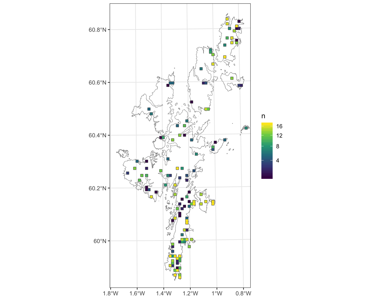
Figure 3.1: Locations and sampling effort of Shetland Breeding Bird Survey, for farmland wader species. Number of years a SBBS 1km square was survyered (n), between 2002 and 2019
3.1.2 Status of population change at survey sites between 2002 and 2019
Before any detailed statistical modelling was undertaken a simple analysis into how the population changed between 2002-2011 and 2012-2019, in each surveyed 1km square (n=139). This gives an initial view as to potential population trends between the two analysis periods.The 1 km squares included were those surveyed in both periods and where farmland waders colonized, increased, remained stable, declined or went extinct. Figure 3.2 shows the status changes between the two analysis periods.
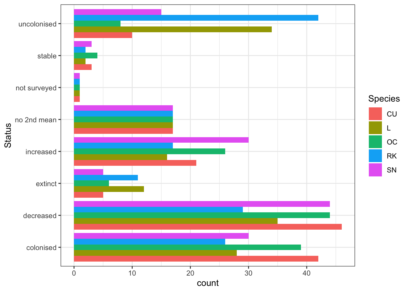
Figure 3.2: Population status change per Shetland BBS square - between 2002-10 and 2011-19
Figure 3.3 below shows an aggregation of certain categories whereby extinct and decreased are grouped, and colonised and increased are grouped. It can be seen that only Lapwing show a net decline over the two analysis periods.
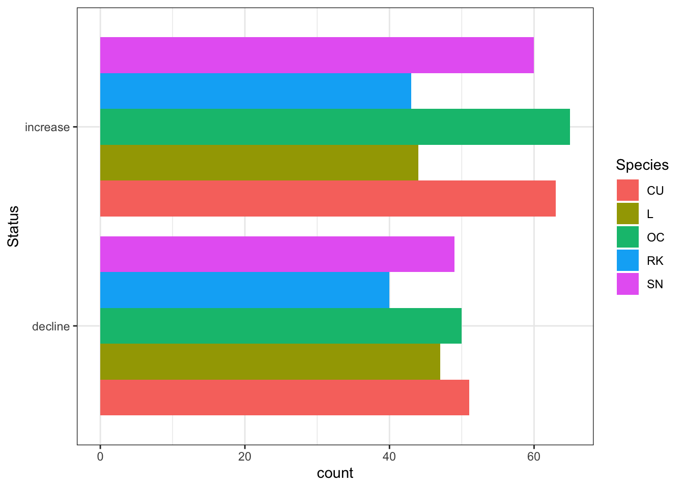
Figure 3.3: Aggregate population status change per Shetland BBS square - between 2002-10 and 2011-19
3.1.3 Outliers
The Cleveland dot plot (Zuur, Ieno, and Elphick 2010) is a chart in which the row number of an observation is plotted versus the observation variable, thereby providing a more detailed view of individual observations than a boxplot. Points that stick out on the right-hand side, or on the left-hand side, are observed values that are considerably larger, or smaller, than the majority of the observations. Figure 3.4 appears to show that there are no significant outliers across all species, but that there are many counts equal to zero indicating that the count data might be zero-inflated.
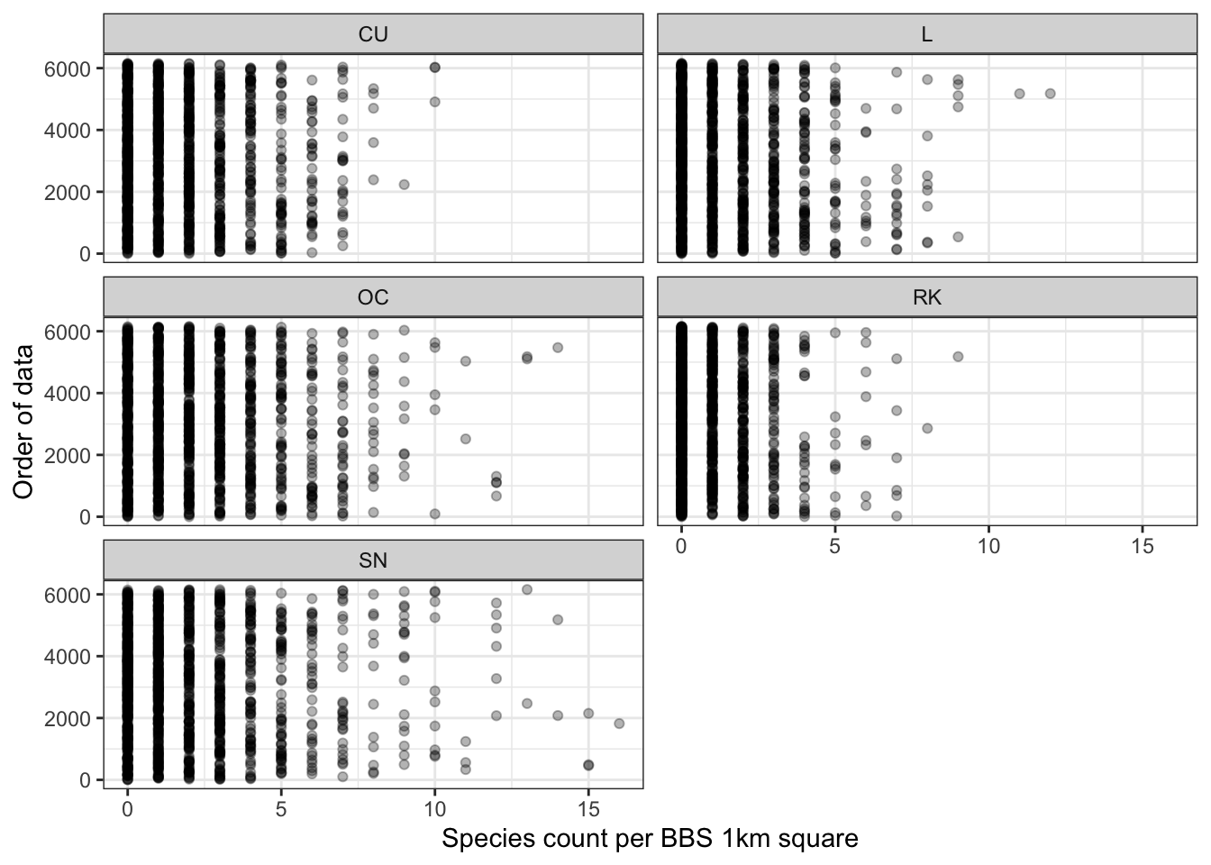
Figure 3.4: Cleveland dot plot of species counts in Shetland BBS data from 2002 to 2019
3.1.4 Testing for normality
A large number of statistical regression techniques assume normality. Visualising the Shetland BBS count data as a histogram can help assess if it is normally distributed. This is shown in the plot in Figure 3.5.
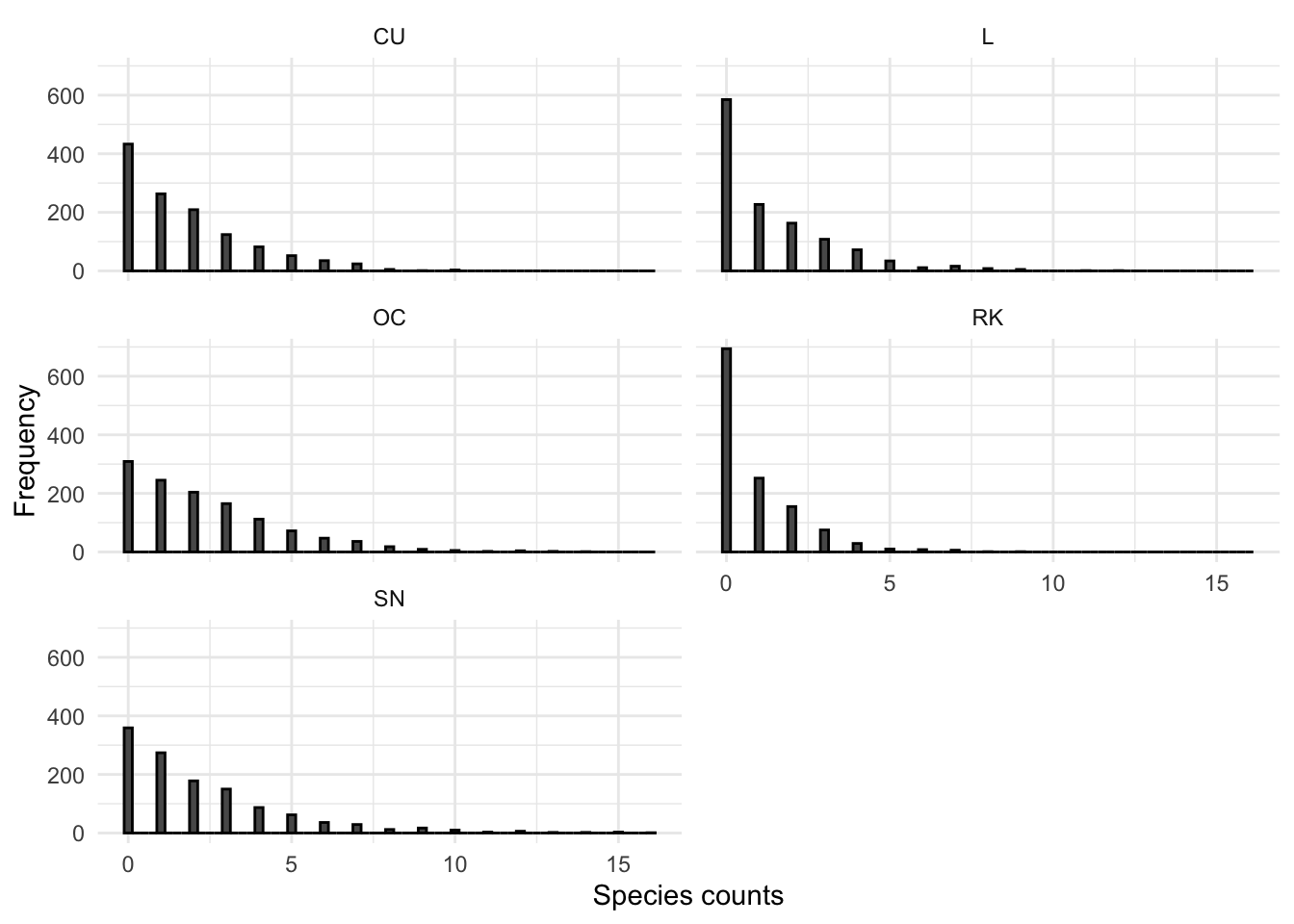
Figure 3.5: Histogram of SBBS count data across all years, by species
Clearly the count data are not normally distributed. In-order to validate the outcome of the plots in Figure 3.5 a Shapiro-Wilks normality significance test was undertaken and the results are shown in Table 3.1.
| Species | W | p-value |
|---|---|---|
| OC | 0.8628058 | 0 |
| L | 0.7546102 | 0 |
| CU | 0.8327195 | 0 |
| RK | 0.6995970 | 0 |
| SN | 0.8000661 | 0 |
The p-value for each species in 3.1 is << 0.05. This suggests that the count data for all species are significantly different from the normal distribution.
3.1.5 Poisson distribution and zero inflation
The histograms of species counts in Figure 3.5 suggest that count data is a poisson distribution. Also there are a significant number of zeros in the count data, across all species count data. This suggests that the zero-inflation poisson distribution describes the data. Table 3.2 below shows the results of a significance test (Broek 1995) for data zero inflation that follow a poisson distribution.
| Species | Expected zeros | Zeros observed | Chi squared | p-value |
|---|---|---|---|---|
| CU | 223.9173 | 433 | 384.2445 | 0 |
| L | 323.5230 | 585 | 547.5071 | 0 |
| OC | 119.1142 | 309 | 446.9641 | 0 |
| RK | 520.3458 | 694 | 271.6801 | 0 |
| SN | 134.4406 | 359 | 577.9990 | 0 |
All results have a significant statistical significance (p<0.05) and therefore the count distribution across species data are assumed to be a zero-inflated poisson process. The statistical modelling methods used on the data must support a poisson distribution and zero inflation where possible.
3.1.6 Homogeniety of variance
Homogeneity of variance within the data is an important assumption in analysis of variance (ANOVA) and other regression-related models. The series of boxplots in Figure 3.6 show how counts across all surveyed BBS squares vary across years 2002 to 2019, for each breeding wader species.
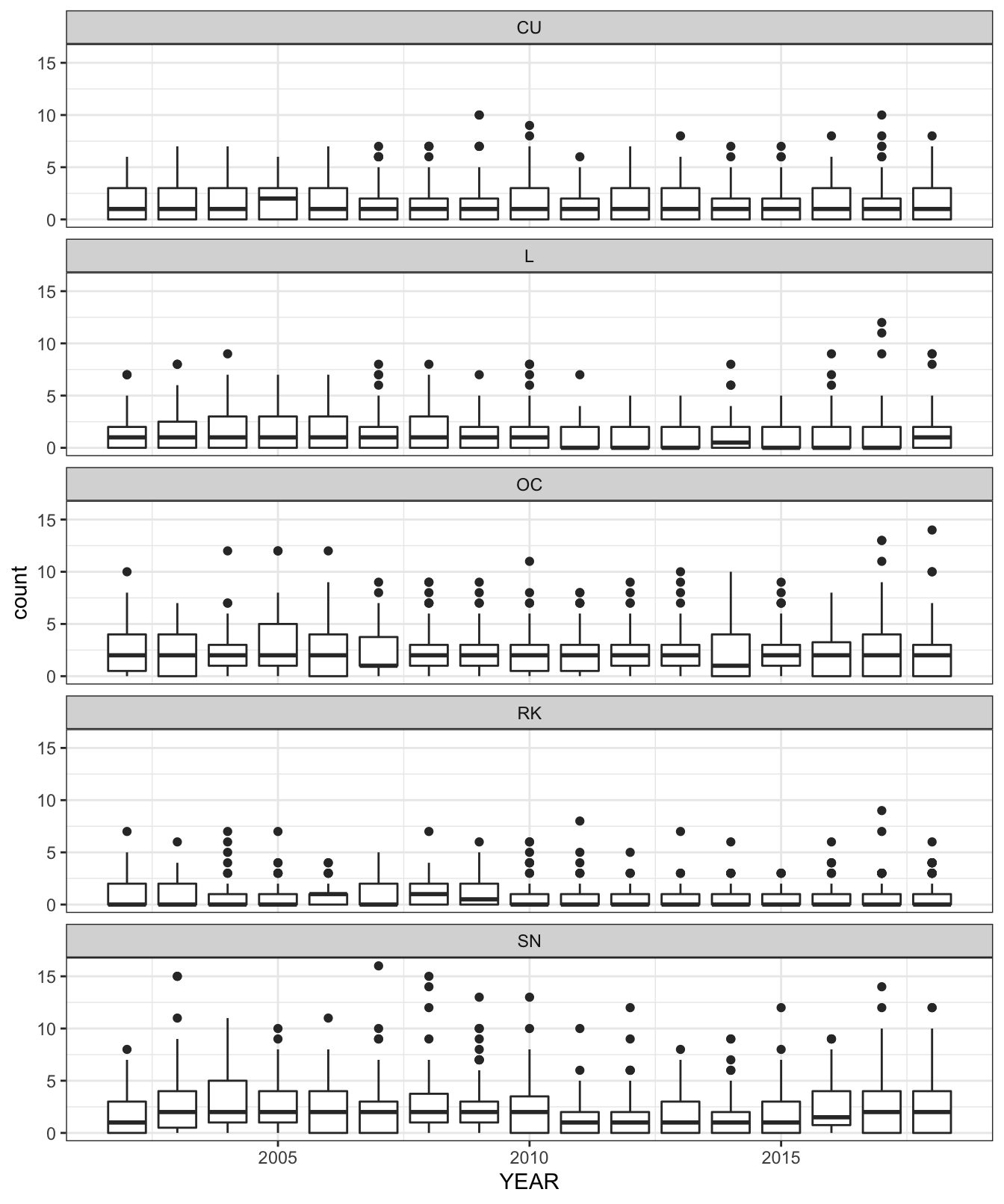
Figure 3.6: Box plot showing variance of counts across all surveyed Shetland BBS squares and all years, by species
To test the homogeneity of variance of species counts between years, for each species, we can apply the Fligner-Killeen test. This is used as the count data are shown to be non-normal. Table 3.3 shows the results of the test applied to the Shetland BBS data. For p-values > 0.05 the data variance are homogeneous.
| Species | Chi-squared | p-value | df |
|---|---|---|---|
| OC | 18.11614 | 0.3171401 | 16 |
| L | 29.11514 | 0.0231712 | 16 |
| CU | 18.36325 | 0.3030590 | 16 |
| RK | 26.72879 | 0.0445979 | 16 |
| SN | 47.40824 | 0.0000588 | 16 |
Lapwing, Redshank and Snipe variances are heterogeneous according to the test results in Table 3.3. The solution to heterogeneity of variance is to transform the response variable to stabilize the variance year-on-year, or applying statistical regression techniques that do not require homogeneity, such as a generalised additive model.
3.1.7 Survey Bootstrap
Shetland BBS volunteers were able to choose which squares they surveyed. As a result of this non-randomised allocation there could be potential bias in the habitat types surveyed; for example, in-by is closer to roads and housing than upland habitats. To test this a bootstrap of percentage cover of EUNIS habitat categories D, E and F (see 2.1) across all Shetland 1km squares was undertaken, and then compared to a bootstrap of the same data, but only those squares surveyed by volunteers as part of the Shetland BBS.
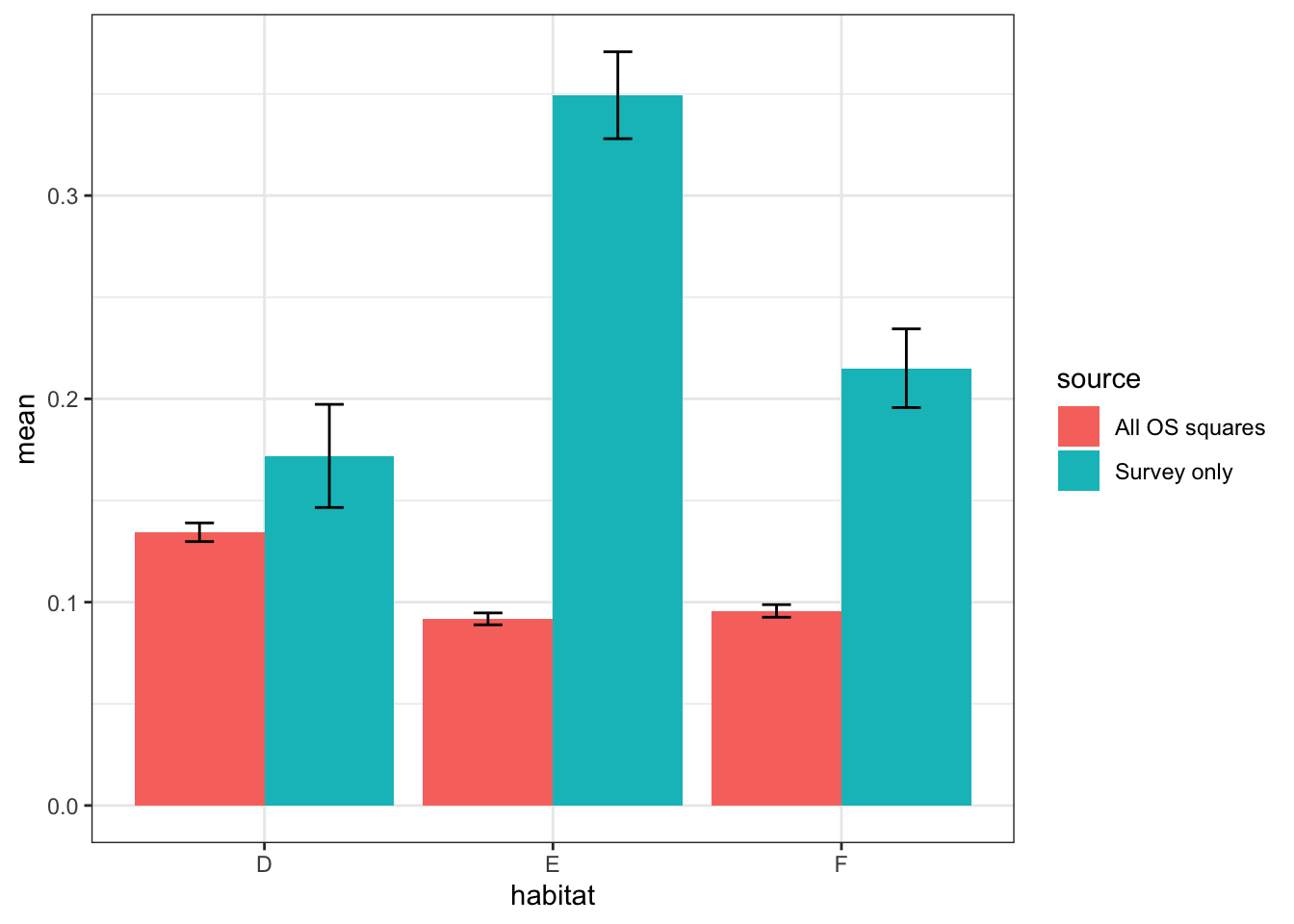
Figure 3.7: Mean % cover per 1km\(^2\) of EUNIS habitat types D, E and F, bootstrap sample of OSGB squares v boostrap of surveyed squares. R=1000
This shows that grassland and heathland are significantly oversampled within the Shetland BBS surveys, but bog habitats appear to be sampled proportionally.
3.2 Detectability
The r package unmarked was used to generate an estimate for the probability of detection, or detectability. Table 3.4 shows the average detectability across all survey years, for each species.
| Species | Detectability |
|---|---|
| OC | 0.803 |
| L | 0.723 |
| RK | 0.667 |
| CU | 0.831 |
| SN | 0.723 |
3.3 Improved grassland classification
The results below detail how remotely sensed satellite data was processed using the Support Vector Machine (SVM) machine learning algorithm to generate a classification for improved grassland across Shetland.
3.3.1 Shetland Sentinel 2 satelitte dataset
A Sentinel 2 Level 2A spatial dataset was clipped using the Integrated Administration And Control System (IACS) (Oesterle and Wildmann 2003) field boundary shapefile for Shetland. This gave a spatial dataset comprising of land-based habitat only, excluding built areas and roads. The RGB composite of the clipped image is shown in Figure 3.8
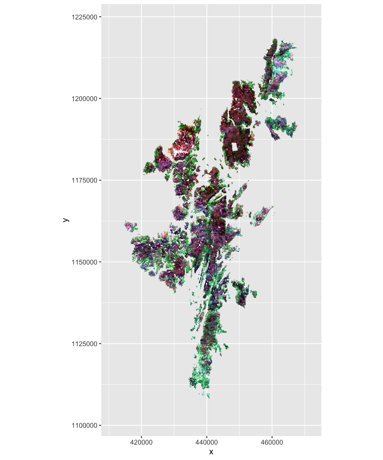
Figure 3.8: Clipped Sentinel 2 RGB composite of Shetland
3.3.2 Habitiat classification training data
In order to classify improved grassland, five other distinctive habitat types were also classified: unimproved grassland, crops, bare peat, cliffs and upland. A number of areas representative of each habitat type were selected as shown in Figure 3.9.
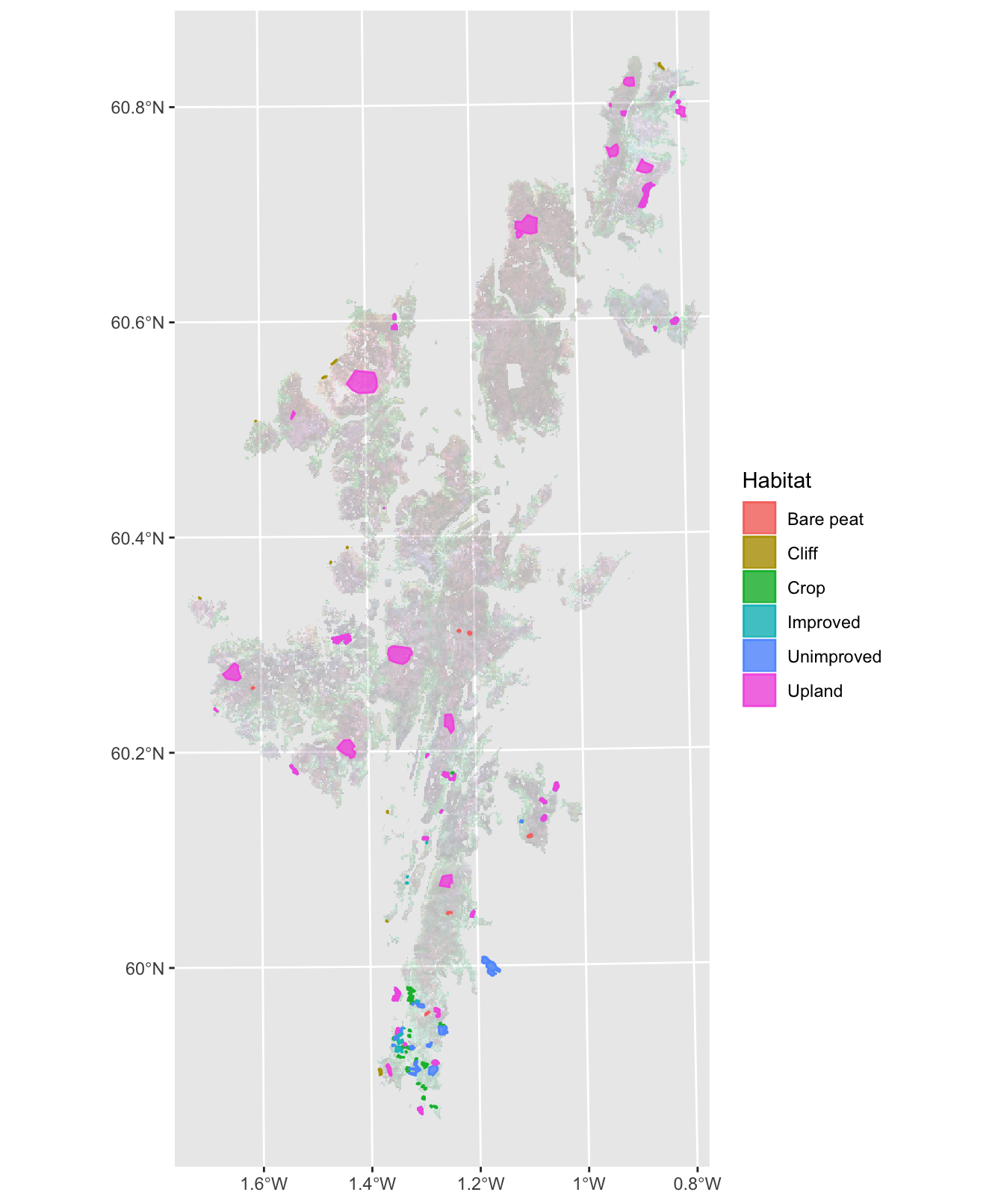
Figure 3.9: Habitat classification training areas
3.3.3 Sampling of habitat training classes
Each habitat training dataset was randomly sampled in order to train the SVM habitat classifier. Distributions for the sampled data for each training set are shown in Figure 3.10.
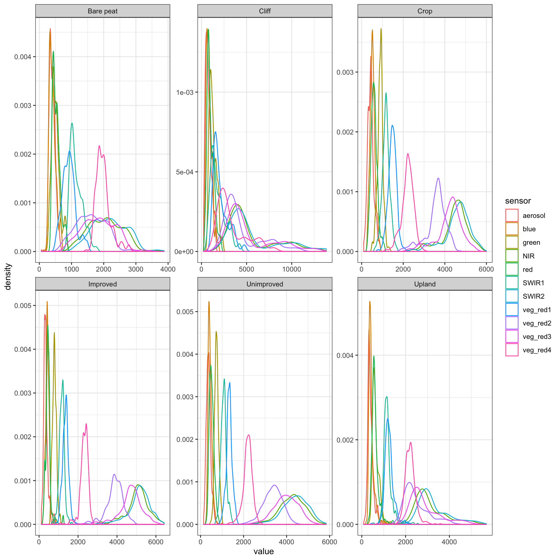
Figure 3.10: Sampled distributions for each training class, from the Sentinel-2 Level 2A dataset of the Shetland archipelago
There are a number of distinguishing observations that can be made from Figure 3.10. Firstly a visual inspection of the bare peat, cliff, upland and crop classes show a clearly different spectral finger-print for each habitat type. Perhaps unsurprisingly improved and unimproved grassland are relatively similar. On closer inspection it can be seen that the shape of the near infra-red (NIR) spectral histogram appears significantly different for improved grassland. A significant proportion of NIR light is reflected by green vegetation, therefore greener “improved” vegetation is likely to have a strong NIR spectral response (Pettorelli et al. 2014).
3.3.4 Support vector machine classifier training
In order to undertake supervised training of an SVM, optimal values for for so-called hyper-parameters must be selected. The type of SVM tuned for classifying improved grassland was a radial basis SVM, and two key hyper-parameters must be tuned for when selecting the best model fit. A so-called search grid is used to specify all permutations of hyper-parameters that will be utilised to find the optimum fit. For the improved grassland classification, the specific search parameters used are shown in Table 3.5.
| RBF sigma | Cost |
|---|---|
| 0.11 | 18 |
| 0.12 | 18 |
| 0.13 | 18 |
| 0.11 | 19 |
| 0.12 | 19 |
| 0.13 | 19 |
| 0.11 | 20 |
| 0.12 | 20 |
| 0.13 | 20 |
3.3.5 Best model results by classification accuracy
The best SVM model hyper-parameters, as measured by classification accuracy, are shown in Table 3.6. It can be seen that when the best model is used to make classification predictions using the training, it achieved an accuracy of 82% with a standard error of 1%.
| Cost | RBF sigma | Accuracy | se |
|---|---|---|---|
| 20 | 0.13 | 0.8233010 | 0.0094407 |
| 19 | 0.13 | 0.8208738 | 0.0093362 |
| 18 | 0.13 | 0.8194175 | 0.0093179 |
| 19 | 0.12 | 0.8194175 | 0.0091478 |
| 20 | 0.12 | 0.8194175 | 0.0090903 |
3.3.6 Model performance using the test dataset
Having selected the best model fit, the same model was used to make predictions against the test dataset. The SVM classifier accuracy was shown to be 85% as shown in Table 3.7.
| Metric | Estimate |
|---|---|
| accuracy | 0.8534091 |
| kap | 0.8240900 |
The confusion matrix in Figure 3.11 shows the results of the model prediction for each habitat class against those of the test data set. The most incorrectly classified habitat is unimproved grassland (class 2) versus upland (class 3), followed by improved grassland (class 1) versus unimproved grassland. This gives an accuracy for improved grassland classification of c.85% over the test dataset.
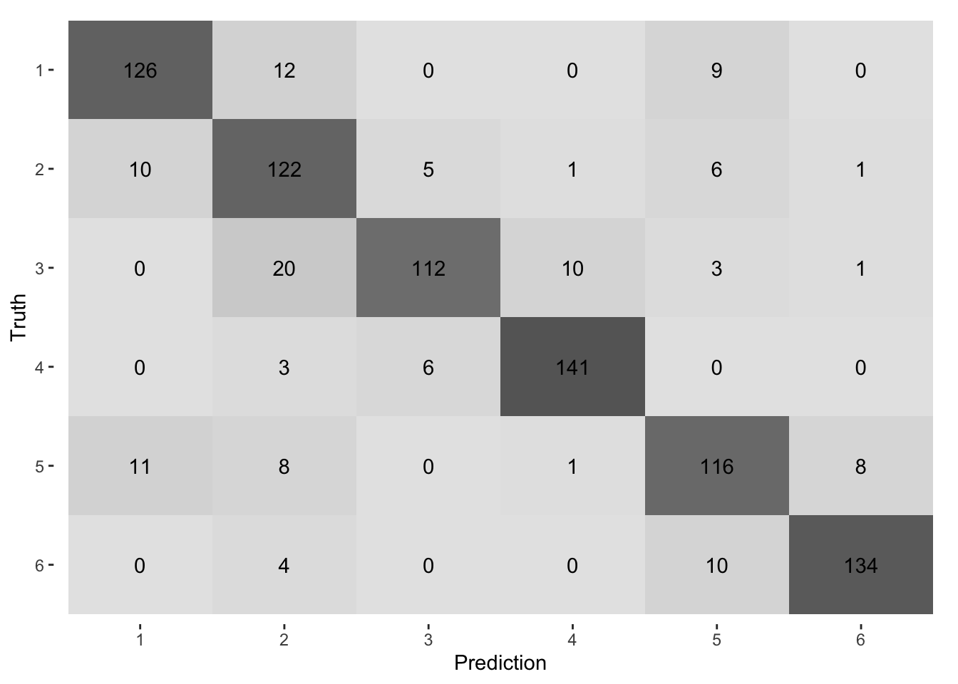
Figure 3.11: Confusion Matrix from classificaton of test dataset
3.3.7 Classification across all Shetland habitat
The best fitting model was used across the entire raster dataset for Shetland, to enable classification of all habitat according to the chosen six habitat classes. The results are shown in 3.12. It can be seen that the improved grassland and crop habitat classes are predominantly in the south of the islands; this was validated by a local expert. It can be seen that the main middle island, Yell, is predominantly upland and bare peat.
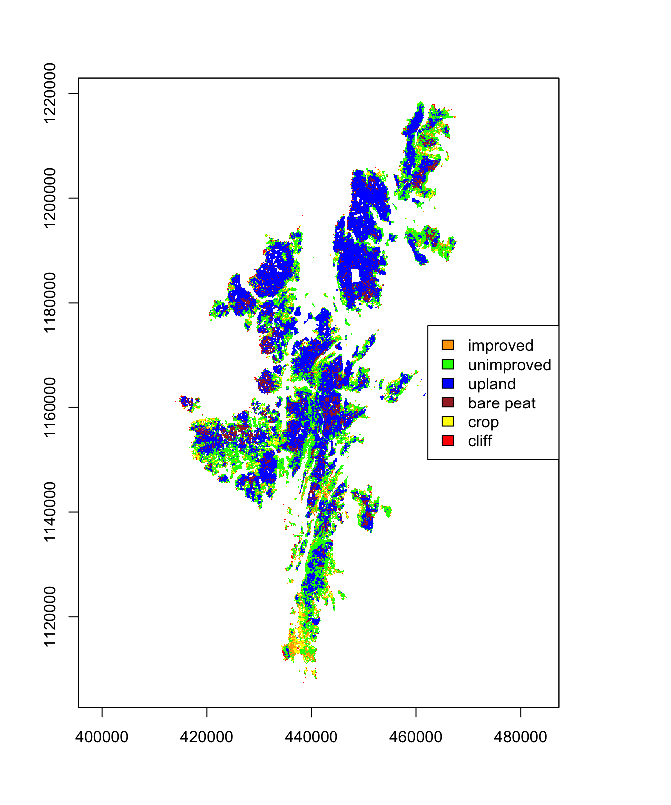
Figure 3.12: Classification of Shetland habitat in order to determine the location of improved grassland
3.4 Environmental covariate analysis
Each of the covariates described in Section 2.4 were generated for each OS 1km Shetland square (n=3992).
3.4.1 Histogram of environmental covariates
Figure 3.13 shows histograms for all environmental covariates across the Shetland archipelago, at 1km resolution. It can be seen that bog type habitat predominates across Shetland, and that majority of the landscape is at less than 100m elevation. The mode for the pH is around 4, which is typical for acidic peatland (Paterson 2011). The topsoil carbon content shows that the majority of the Shetland soils have a high organic carbon content; again this is typical of peatland (Paterson 2011). In contrast a typical mineral rich soil in southern England would have c.3-5% organic carbon content. Note that the percentage landcover of improved grassland is relatively low compared to the more general grassland classification. This shows that agricultural intensification is relatively low in Shetland.
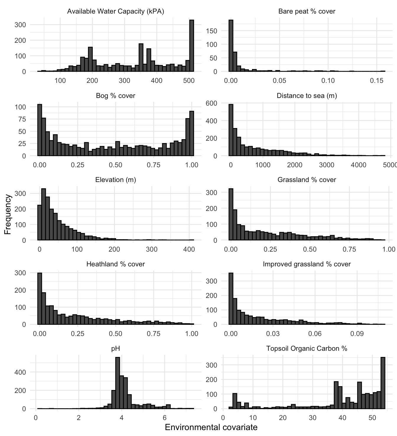
Figure 3.13: Histograms of environmental covariates across all of Shetland
3.4.2 Histogram of environmental covariates for Shetland BBS squares only
This can be contrasted with covariate histograms for only those OS squares (n=139) that were surveyed as part of the Shetland BBS, as seen in Figure 3.14. If these data are indicative of general breeding wader habitat preferences, it would seem that across all surveyed nesting wader species, there is a preference for wet but not water-logged habitat as seen in the AWC histogram. Also, the majority of breeding waders that were surveyed appear to nest within 1km of the coast. It appears that surveyed breeding waders also have a preference for grassland (both improved and unimproved) presents the majority of the habitat cover, over heathland.
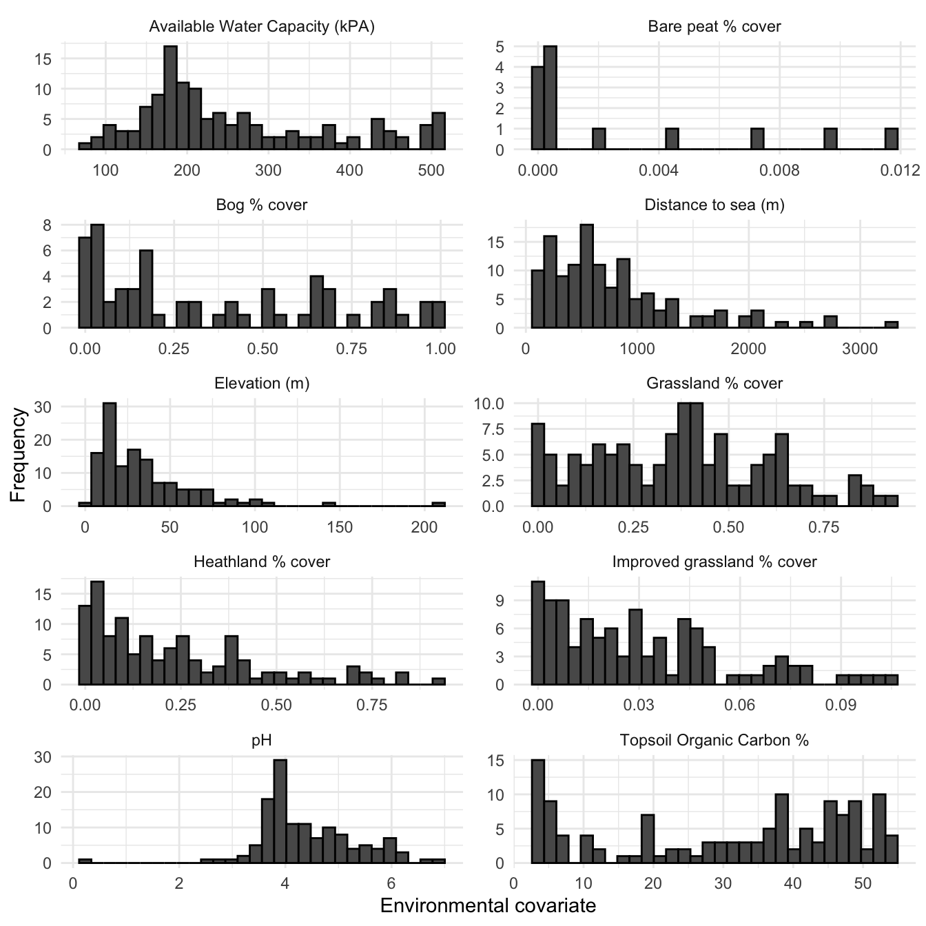
Figure 3.14: Histograms of environmental covariates across only those squares surveyed as part of the Shetland BBS
3.4.3 Density plots of environmental covariates
Density plots of all environmental covariates across Shetland BBS squares (n=139) are shown in Figure 3.15. These figures provide an overlay to the histograms in Section 3.4.2, and represent a smoothed version of a histogram to show the probability density function of the variable. Some distributions are highly skewed, such as distance to sea and elevation. Whilst other covariates like topsoil organic carbon and bog cover are largely a uniform distributed. None of the covariates appear to be normally distributed.
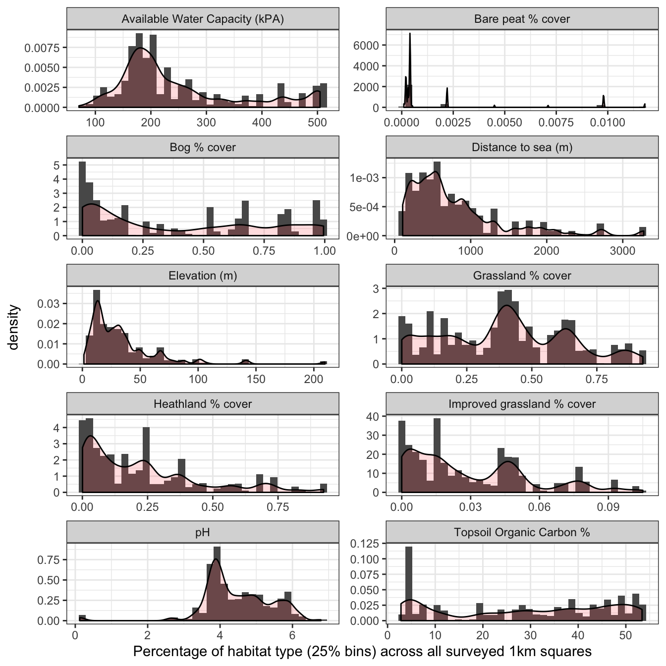
Figure 3.15: Density plots of environmental covariates against breeding wader count data
3.5 Breeding wader abundance response to environmental covariates
Generalised Additive Models (GAMs) for breeding wader abundance response across the five different species were generated from 2002–10 and 2011-19. A GAM was produced for each of the 10 environmental covariates (predictor variables), and for each of the two analysis periods.
Appendix B details the GAM parameter results from the model fitting process, for the two periods where the abundance response (density) was modelled against environmental covariates. The associated plots showing breeding wader density response against each environmental covariate are shown in Appendix C. Note those models that result in a parametric term (an environmental covariate) that is statistically significant (p<0.05) have plots that are coloured red. The statistically significant correlations between breeding wader density and environmental covariates are summarised for each species in heatmaps; Figure 3.16 for 2002-10 and Figure 3.17 for 2011-2019.
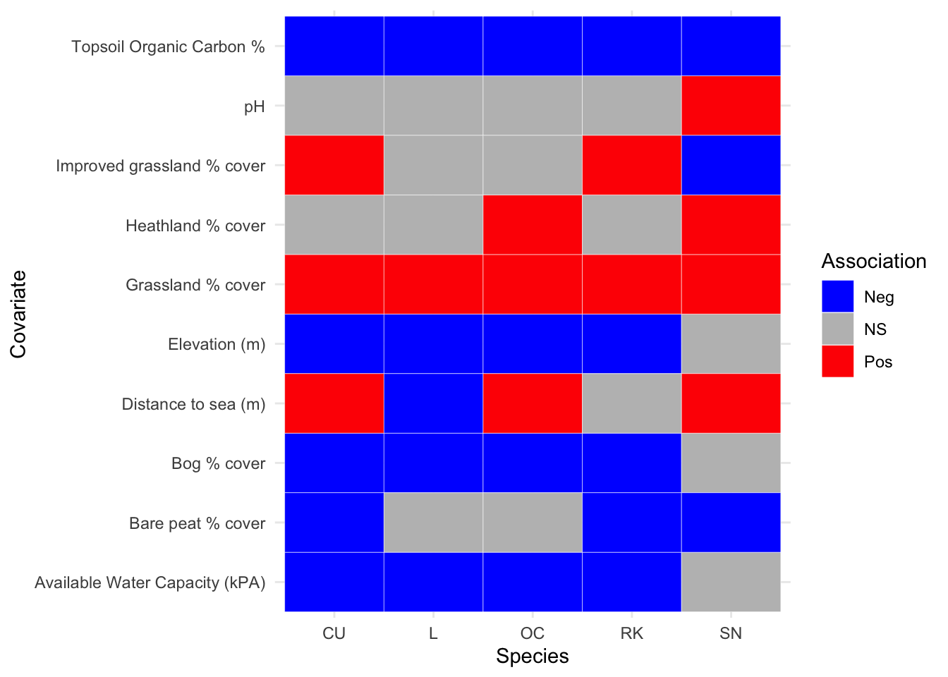
Figure 3.16: Summary of associations between breeding wader density and environmental covariate, between 2002 and 2010 inclusive
For the 2002-10 survey period in Figure 3.16, it can be seen that pH is only statistically significant for one species (Snipe), whilst topsoil organic carbon and grassland are oppositely correlated. Distance to sea is perhaps the most interesting covariate in that Lapwing show a greater association at the coast whilst Curlew, Oystercatcher and Snipe show greater densities inland. Notable results are that all nesting species are negatively associated with higher percentages of carbon within the topsoil per km\(^2\), and all nesting species are positively associated with increased grassland coverage per km\(^2\).
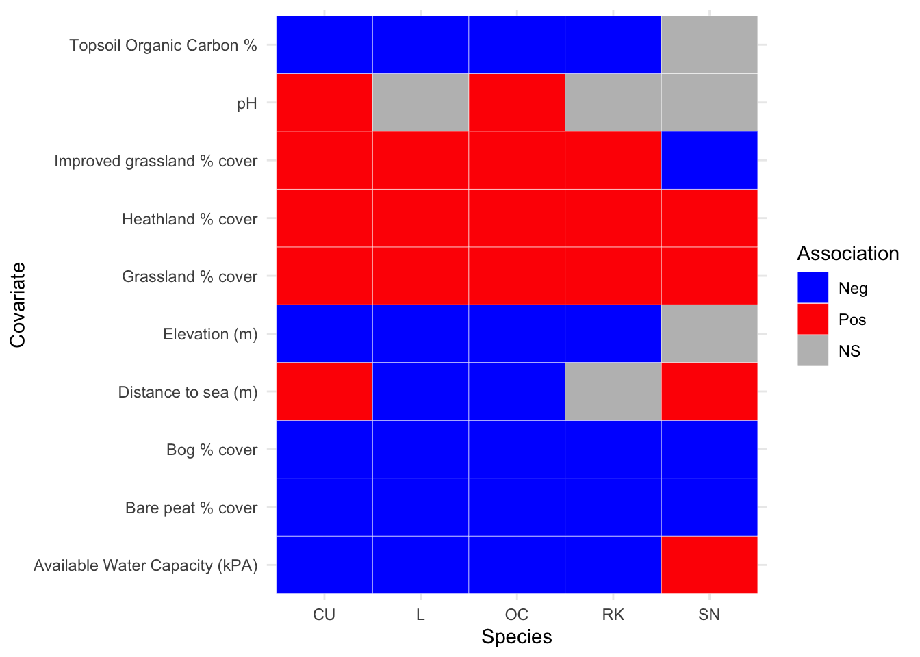
Figure 3.17: Summary of associations between breeding wader density and environmental covariate, between 2011 and 2019 inclusive
In Figure 3.17 we can see that there are fewer associations that are not statistically significant. Again all species are positively associated with increased grassland coverage per km\(^2\), and in the second analysis period this is true for increased heathland coverage per km\(^2\). All species are now negatively associated with increased bog coverage per km\(^2\) and increased bare peat coverage per km\(^2\). It can also be seen that all species, apart from Snipe, are positively associated with increased improved grassland coverage per km\(^2\). Where as the exact opposite is true for available water capacity per km\(^2\).
For Curlew it is seen that all covariate associations are now statistically significant (versus 2002-2010 where pH and Heathland cover were not significant). Oystercatcher also have all covariates with statistically significant associations. Note that for Oystercatcher, for the second analysis period, results for the distance to sea association show a negative association with increasing distance. Lapwing only have one covariate, pH, that is not statistically significant, and otherwise show identical results to Oystercatcher. For Redshank the main change in the later analysis period is that Heathland percentage cover is now statistically significant, and has a positive association. Snipe now have a positive association with available water capacity and a negative association with percentage bog cover.
3.6 Population change response against environmental covariates
A third model was generated by using the abundance response from the first two GAMs in Section 3.5. By using the response of the 2002-2010 wader densities as the offset for the 2011-19 densities, a third series of GAMs were fitted to show the ratio of population change as a function of environmental covariates. The population change model will give an indication of how breeding wader densities have changed over time for a given environmental covariate. For example, are species decreasing over time in habitats that are thought to offer lower food availability for chicks, such as heathland.. The results of the analysis are shown in Figure 3.18.
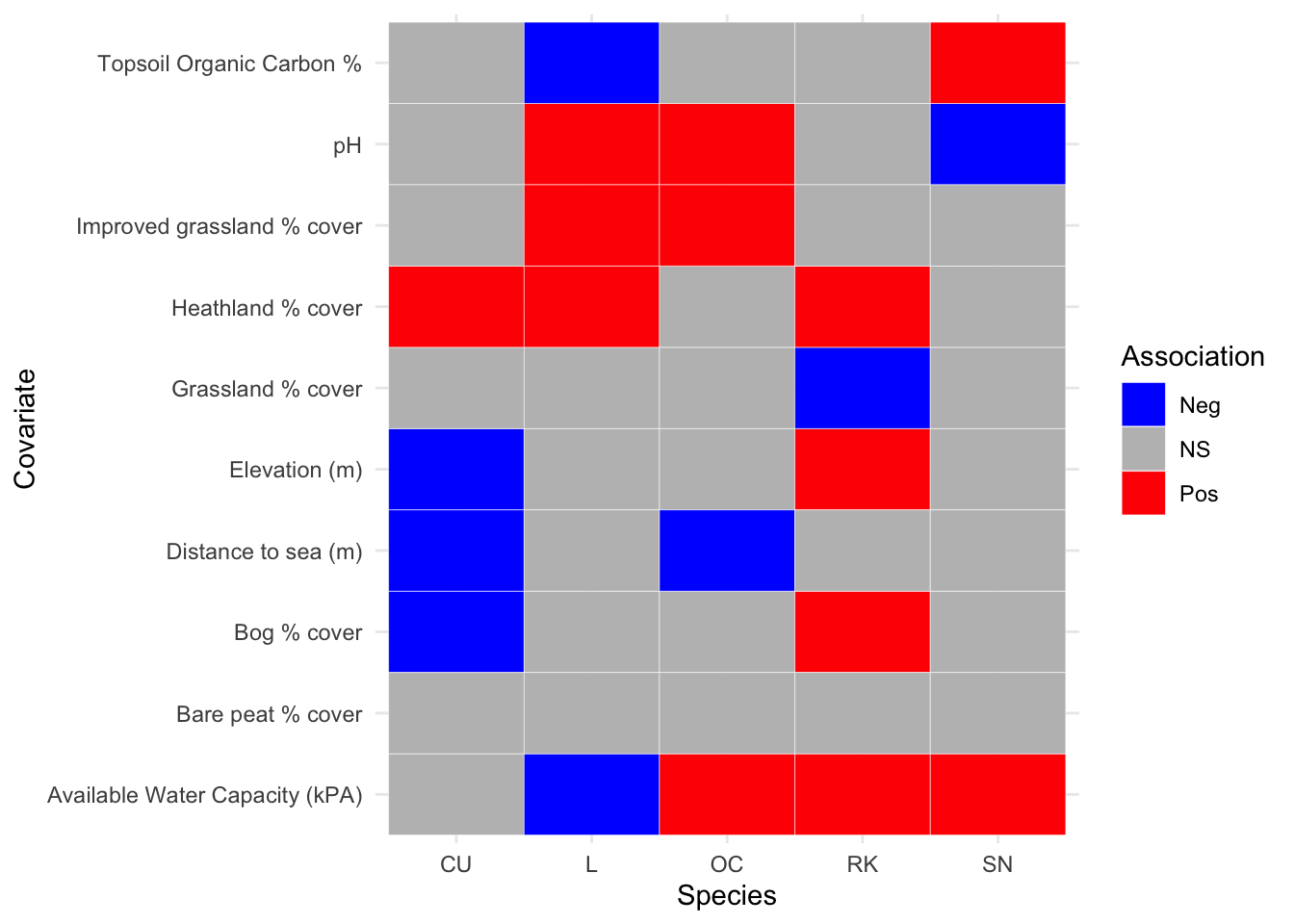
Figure 3.18: Summary of population change ratio associations between breeding wader density and environmental covariate, between 2002 and 2019 inclusive
Figure 3.18 suggests that the environmental covariates that have had the most positive associations with breeding wader population changes over the two analysis periods are heathland percentage cover and available water capacity. The percentage of bare peatland has had no statistical significance, followed by the percentage grassland cover that has only one negative association with the population change ratio of Redshank. The model parameters and associated plots for population change ratio modelling are shown in Appendix D and Appendix E respectively.
3.7 Information Theory (IT) covariates
GAMs for breeding wader abundance response across the five different species were generated from 2002–10 and 2011-19. In addition to the environmental covariates, they included five IT covariates. The model parameter results for all species across the two analysis periods can be seen in Appendix F. A third model was generated by taking the abundance response from the first two models to generate the ratio of population change between the two response periods, the model parameters for this model can be seen in Appendix @ref{#gam-it-pop-chg-params}.
3.7.1 Histograms of Information theory covariates
Histograms of IT covariates using the EUNIS landscape categorisation, across all of Shetland are shown in figure 3.19. The marginal entropy for the Shetland landscape is approximately normally distributed, indicating that habitat within the Shetland landscape is spatially diverse but that very low and highly diverse habitat within Shetland are relatively rare. The mode of the conditional entropy is relatively low with a distribution that shows significant positive skew; this suggests that the Shetland landscape has relatively low geometric intricacy. This arises when cells of one category within a landscape raster are predominantly adjacent to cells of the same category. The overall spatio-thematic complexity is measured by the joint entropy. This can be thought of as quantifying the uncertainty in determining the habitat type of a focus cell and an adjacent cell. For Shetland, joint entropy appears to be approximately normally distributed. This indicates that habitat with very high or low spatio-thematic complexity is relatively rare on Shetland. Due to the spatial autocorrelation, the value of mutual information tends to grow with a diversity of the landscape (marginal entropy). To adjust this tendency, it is possible to calculate relative mutual information by dividing the mutual information by the marginal entropy. Relative mutual information always has a range between 0 and 1, and quantifies the degree of aggregation of spatial habitat. It can be seen that for Shetland, relative mutual information is distributed with significant negative skew. This implies that habitat types across Shetland are predominantly aggregated - small relatively information values indicate significant fragmentation in landscape habitat patterns.
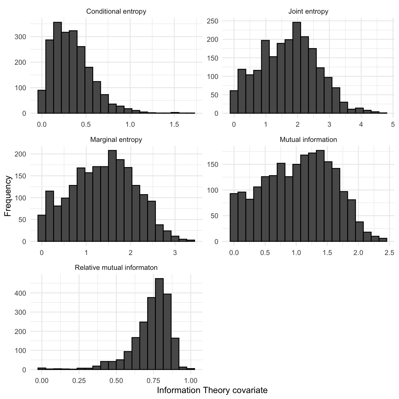
Figure 3.19: Histograms of Information Theory covariates across all Shetland OS 1km squares
3.7.2 Histograms of Information Theory covariates for surveyed squares only
1km squares surveyed as part of the Shetland BBS were used to generate IT covariates histograms using the EUNIS landscape categorisation, as shown in Figure 3.20. Here we can see that the conditional entropy and the marginal entropy across all surveyed squares had a mode that was significantly higher than the Shetland wide values shown in Figure 3.19. There is also significantly less negative negative skew in the relative mutual information of the surveyed squares.
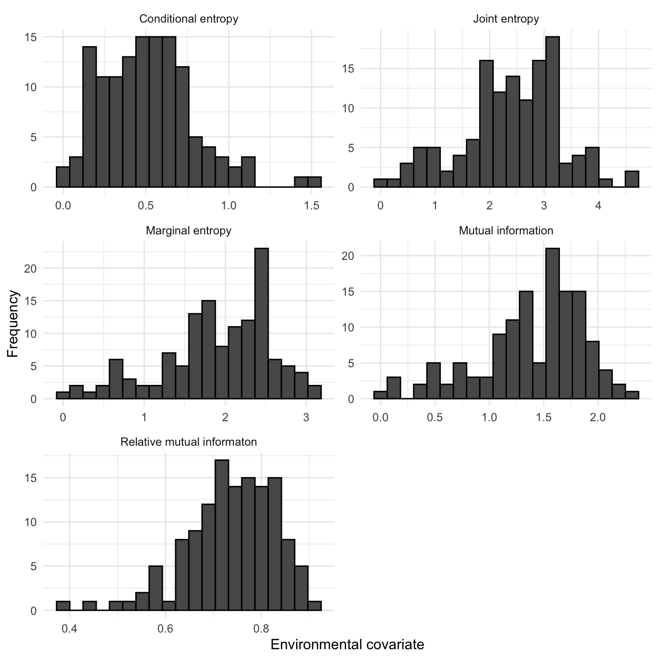
Figure 3.20: Histograms of Information Theory covariates across SBBS surveyed sqaures only
3.7.3 Information Theory covariates abundance response model
GAMs were fitted for each of the two analysis periods using IT metrics as covariates against breeding wader abundance. Figures 3.21 and 3.22 summarise the associations between the abundance response and IT covariates used in the univariate GAMs, for the periods 2002-10 and 2011-19 respectively.
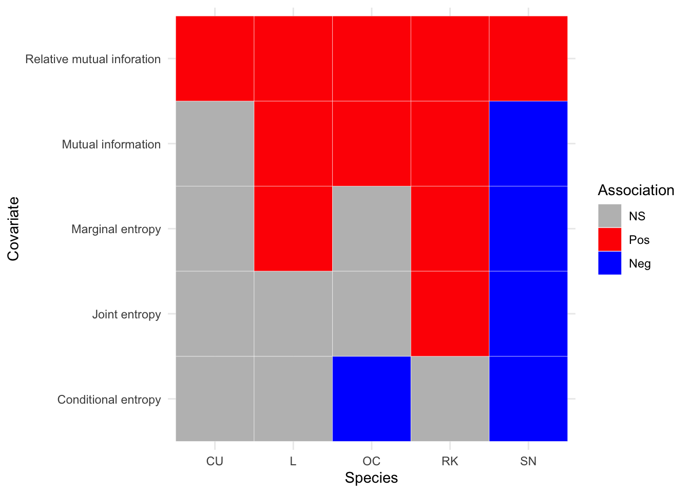
Figure 3.21: Summary of associations between breeding wader density and IT covariates, between 2002 and 2010 inclusive
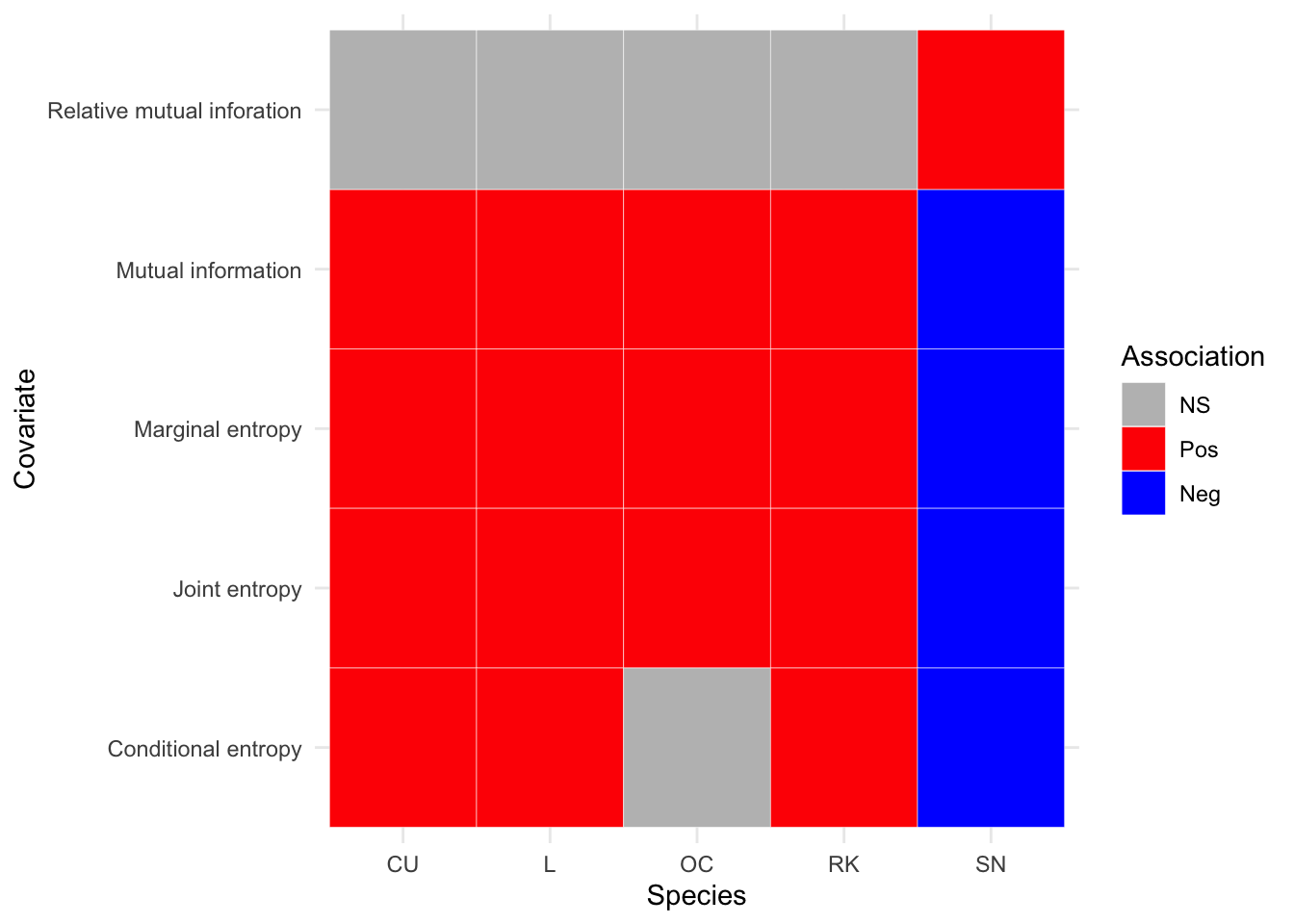
Figure 3.22: Summary of associations between breeding wader density and IT covariates, between 2011 and 2019 inclusive
Appendix F shows the GAM parameter results generated by fitting the model to the data when information theory metrics are used as covariates. Plots showing the abundance response against IT covariates are shown in Appendix G.
It seems that the response for Snipe abundance to IT covariates is identical for the two periods. Snipe have a positive association with relative mutual information, or habitats that have a high degree of aggregation, such as heathland. Relative mutual information has no statistically significant association for any other species in the second analysis period, although it appears to be statistically significant and positively associated for all species in the first analysis period. This indicates that breeding waders, apart from Snipe, may have moved from areas comprising habitat that is highly aggregated to areas that are less so. This hypothesis is partially supported by the fact that the second analysis period shows increase in wader species, apart from Snipe, that are positively associated with marginal entropy; a measure of habitat thematic diversity.
3.7.4 Population change model against IT covarirates
By using the response of the 2002-2010 wader densities as the offset for the 2011-19 densities, a third series of GAMs were fitted to show the ratio of population change in response to IT covariates. This is summarised in Figure 3.23. It can be seen that there are no statistically significant results for Redshank or Snipe, or for marginal entropy as a covariate.
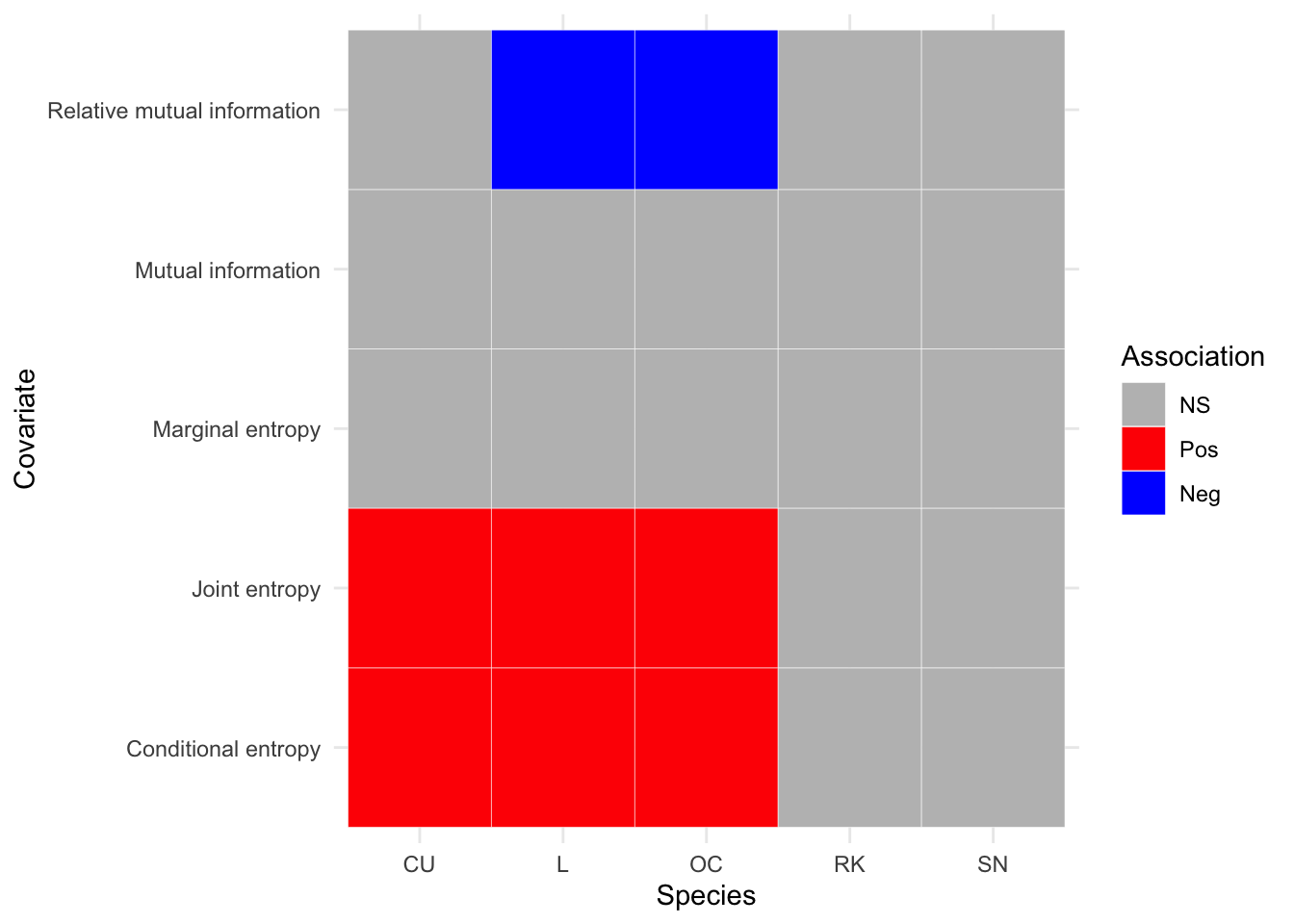
Figure 3.23: Summary of associations between breeding wader density and IT covariates, between 2011 and 2019 inclusive
Perhaps the most significant result is that which supports the idea that breeding wader densities have declined in habitats that exhibit a large spatial aggregation. This is shown by the fact that Lapwing and Oystercatcher populations are negativelty associated over time, with increased relative mutual information. Appendix H shows the GAM parameters generated by fitting the population change model to the data. Plots for population change response against IT covariates are shown in Figure I.
3.8 Wader abundance trends
A random forest regression model was used to fit an abundance response using all 10 environmental covariates. The parameterisation and results are outlined below.
3.8.1 Tuning the model hyper parameters
A search grid over 10 different folds gave initial results for various permutations of hyper parameters as shown in Appendix J. Each figure shows the results for a particular species. Each hyper-parameter permutation is plotted against the resulting root mean squared error (rmse).
3.8.2 Further model hyper parameter tuning
Given the initial results in J the initial range over which the hyper-parameter search was conducted, was refined further by searching over a revised range according by selecting upper and lower limits for hyper-parameters that gave the lowest rmse as indicated by the initial results. The range used was that which gave the lowest rmse as given in Appendix J. The results of the revised search grid range can be seen in Appendix K. Again each plot is for a separate species.
From the plots in Appensix K we can see which hyper parameters give the best fit, when using root mean squared error as an evaluation metric. It can be seen that the model fit for Snipe has the largest RMSE. whilst Redshank has the lowest. For each species the minimum rmse result for the best model fit, together with the associated hyper parameters (trees= 1000 for all models) is shown in Table 3.8.
| Species | mtry | min_n | rmse |
|---|---|---|---|
| CU | 4 | 6 | 1.448835 |
| L | 5 | 4 | 1.672523 |
| OC | 4 | 10 | 1.845994 |
| RK | 7 | 3 | 1.429948 |
| SN | 2 | 6 | 2.718174 |
3.8.3 Variable importance in model fit
Having selected the best model fit the variable importance for each species was assessed. The r package vip (Greenwell, Boehmke, and Gray 2020) was used to explore the relative importance of different covariates in the model fit. The results are shown in Appendix L.
It can be seen that pH, X (longitude) and grassland percentage coverage for a given OS 1km square appear to be the most important covariates for predicting abundance in Curlew. For Lapwing, pH, heathland percentage coverage and topsoil organic carbon content are the most important variables. Whilst for Oystercatcher, grassland and heathland percentage cover are almost equivalent in their importance followed by longitude. For Redshank and Snipe, available water capacity and heathland are the most important covariates in predicting abundance.
3.8.4 Breeding wader population estimates from 2002 to 2019
The random forest regression model was used to predict species abundance over all (n=3992) Shetland BBS 1km squares. The model gave a mean estimate together with lower and upper confidence intervals (5% and 95% percentiles respectively), across every year the survey was run (2002 to 2019). The population estimate results are shown in Appendix M and plotted in Figure 3.24
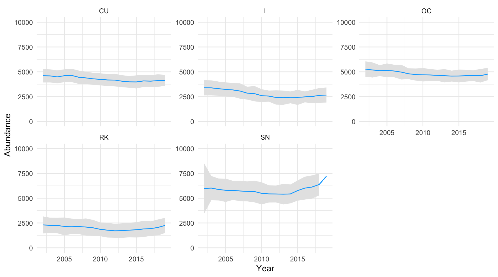
Figure 3.24: Breeding wader population estimates - number of pairs of breeding waders by species, 2002 to 2019. Grey shaded area indicates upper and lower confidence intervals
Across the years 2002 to 2019 the abundance of breeding wader pairs across all species appear to have decreased, with the exception of Snipe. The most significant decline was for Lapwing. Note that the confidence intervals for Snipe are highly variable in certain years. Table 3.9 shows the change in breeding wader abundance by species between 2002 and 2019.
| Species | 2002 | 2019 | % Change |
|---|---|---|---|
| CU | 4597 | 4088 | -11.1 |
| L | 3474 | 2638 | -24.1 |
| OC | 5269 | 4760 | -9.7 |
| RK | 2390 | 2248 | -5.9 |
| SN | 6043 | 7391 | 22.3 |
3.8.5 Lapwing abundance association with grassland holdings
Data from 2002 to 2017 for grassland holdings in hectares categorised as: tillage, grassland less than five years old (reseeded grassland), grassland five years or greater and private grazing were tested for normality, and found to be log-normally distributed. A linear regression was plotted for Lapwing abundance versus each grassland categorisation (in Hectares) as shown in Figure 3.25.
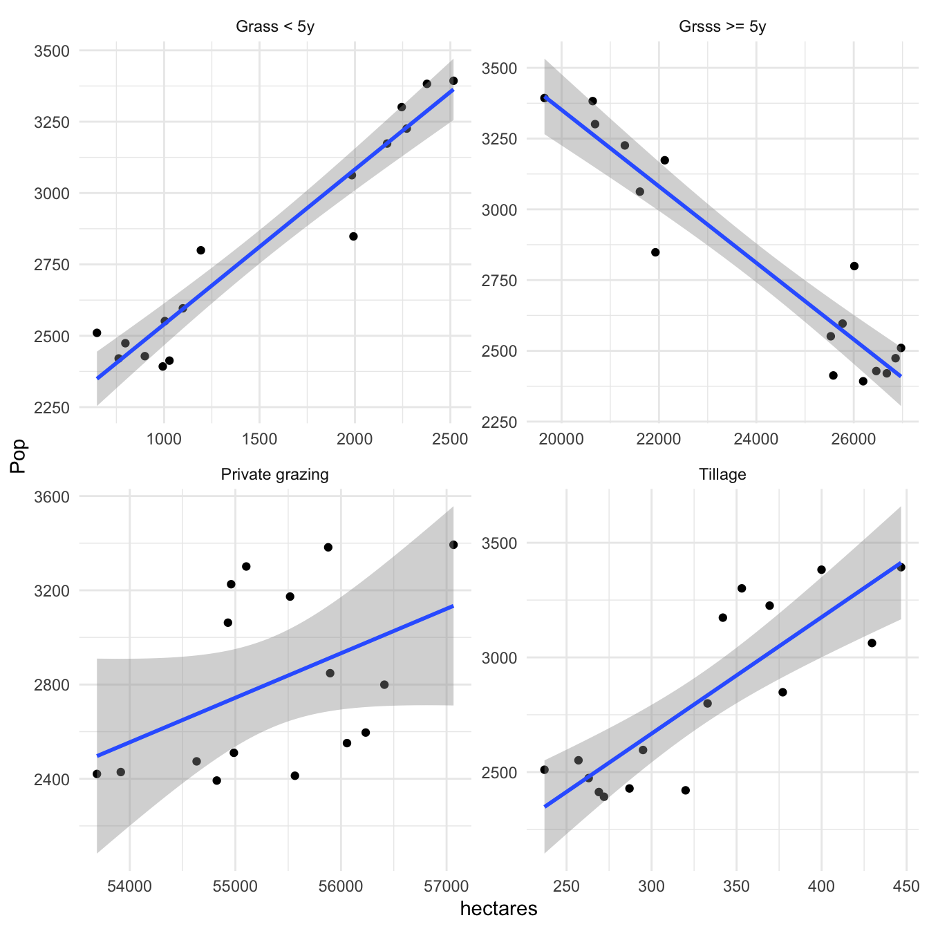
Figure 3.25: Association between the size of grassland categories on Shetland and Lapwing population abundancebetween 2002 and 2017. Agricultural statistics taken from Scottish Agricultural Survey
Figure 3.25 shows that Lapwing population size is positively associated with the size of grassland that is less than five years old (that grassland which has been reseeded) and tillage (land prepared for spring crops). Figure 3.25 also shows that Lapwing population abundance is negatively associated with grassland that is not reseeded (Grass >= 5y).
The r package gamlss (Rigby and Stasinopoulos 2005) was used to fit a log-normal model for Lapwing population abundance with grassland less than 5 years old as a covariate. The grassland < 5 years old was a statistically significant covariate (p<0.0001), and the residuals of the model were approximately normally distributed as shown in Figure 3.26.
## GAMLSS-RS iteration 1: Global Deviance = 192.9757
## GAMLSS-RS iteration 2: Global Deviance = 192.9757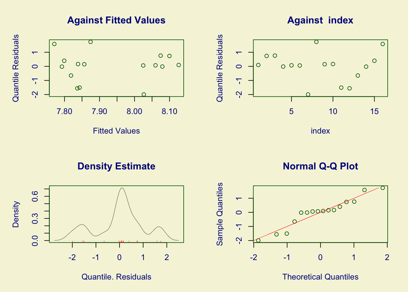
Figure 3.26: Residuals for model fit of Lapwing population estimates to Shetland improved grassland less than five years old. Agricultural statistics taken from Scottish Agricultural Survey
3.9 Spatial abundance distriution of breeding waders
The population estimates results in 3.8.4 are based on a spatial prediction. As such they can be plotted to show how species abundance is spatially distributed across Shetland. Figure 3.27 shows the abundance distribution, per 1km\(^2\) (density) for each species in 2019.
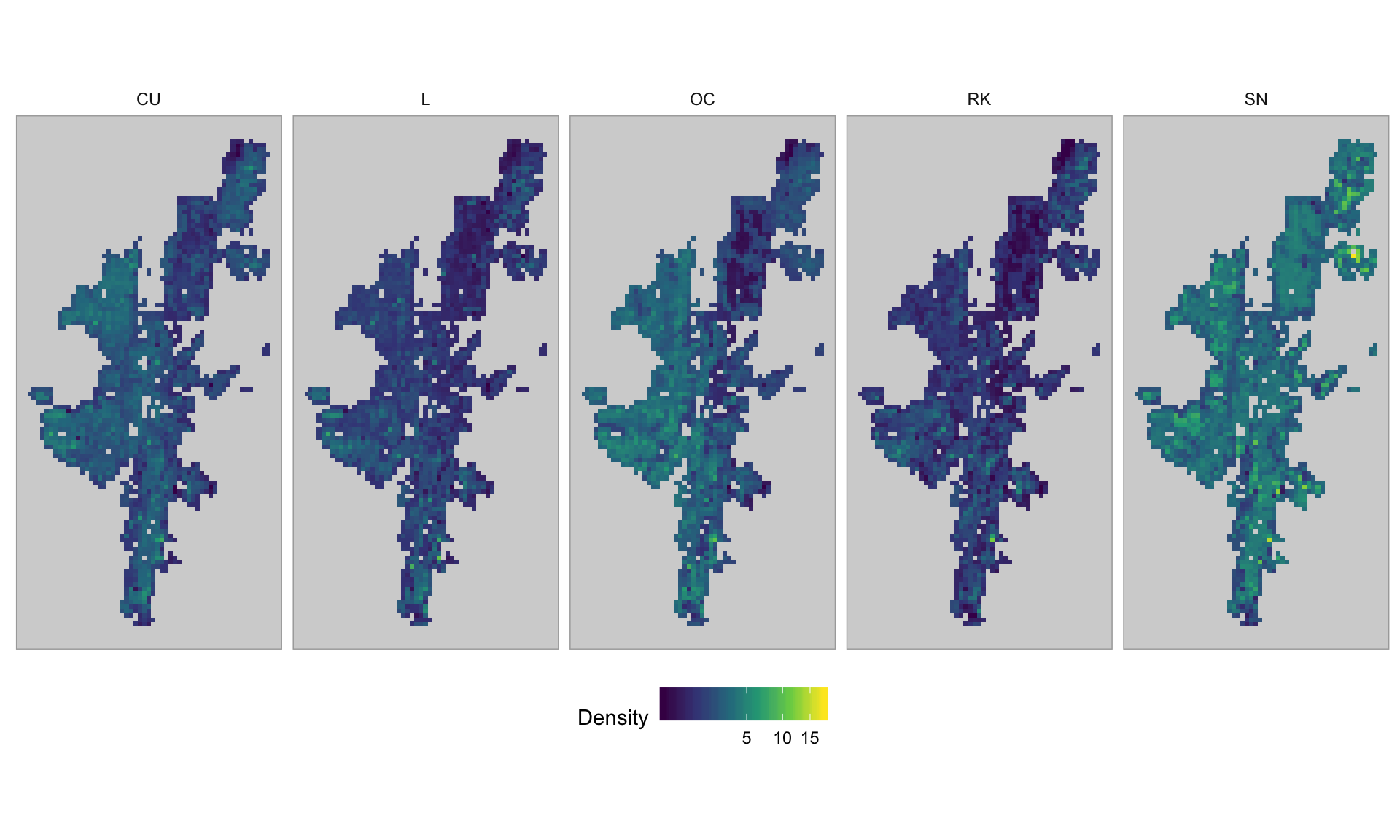
Figure 3.27: Spatial abundance distribution of breeding waders for 2019
It can be seen that Snipe are widespread, and that Curlew and Oystercatcher are significantly present on the western side of Shetland, as suggested by the variable importance plots in Appendix L. Lapwing and Redshank have the lowest population densities and seem to be concentrated in the south west of Shetland.
3.9.1 Net spaital abundance change by species, between 2002 and 2019
Given the spatial abundance distribution for 2002 and 2019, it is possible to plot the net change in breeding wader abundance, for each 1km\(^2\), between the two years. This is shown in Figure 3.28.
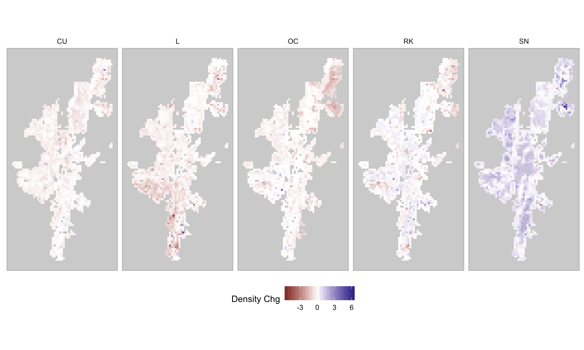
Figure 3.28: Change in breeding wader density (count/km2) between 2002 and 2019 on Shetland
It can be seen that the drop in abundance as shown in Appendix M is reflected in the net change plots in Figure 3.28.
The initial analysis of the status of surveyed 1km squares (see Figure 3.3) suggested that Lapwing had undergone a decline, and Figure 3.28 shows that this has occurred in the south west and north east over the two analysis periods. Oystercatcher appear to have undergone a significant decline in the north east of Shetland (the islands of Unst and Fetlar). Where as Snipe appear to have increased in most upland areas of Shetland, and in particular on the Fetlar RSPB reserve.