2 Materials and Methods
2.1 Shetland Breeding Bird Survey
The Shetland Breeding Bird Survey (BBS) is a citizen science project that is overseen by the Shetland Biological Records Centre (Harvey 2002), the primary objective of which is to assess the population trends Shetlands more common breeding song birds and waders. The survey has been ongoing since 2002, where 36 local volunteers surveyed a total of 49 1km Ordnance Survey 1km\(^2\) squares. It is important to note that to encourage volunteer uptake, these squares are not randomly allocated in space; typically the location of the survey is selected by the volunteer. There are 3992 1km squares that cover the Shetland archipelago; excluding Fair Isle and Foula. A significant proportion of these squares only partially cover the landscape, hence why there are 3992 1km squares to cover the 1,466 km\(^2\) area of Shetland.
When under taking the Shetland BBS volunteers walk either a 2km transect around their chosen square, or two 1km transects that bisect the square. All breeding bird species observed 100m either side of the transect are recorded by the volunteer. All transects were walked twice, typically April to mid-May and mid-May to late June. All surveys were undertaken before 9am and in good weather (wind force four or less, and dry). The annual abundance recorded for each breeding species within a given square is the maximum count from the two separate visits. Upto 2019 there have been 139 different OS 1km squares surveyed as part of the SBBS. Although the survey runs every year, not all 139 survey squares have been covered annually. Since 2002, new squares have been introduced over the years, some are no longer covered, and there are some gaps when volunteers have been unable to carry out surveys.
2.2 Estimating detectability
The Shetland BBS assumes perfect detectability of the survey species. Due to the imprecise nature of field surveys this could result in a bias in species detectability, which could further result in inaccurate population estimates. To account for this bias, there are a number of more sophisticated survey techniques such as distance sampling that account for this, in order to reduce the standard error associated with a population estimate (Newson et al. 2008). Such techniques typically require more structured survey techniques such as precisely measuring the distance and angle, between the target species and the transect line. Unfortunately this data was not available for the two survey datasets used within the study. In-order to generate a probability of detection, and therefore account for detectability bias, the r package unmarked (Fiske and Chandler 2011) was used to generate a probability of detection for each species. Unmarked adopts a generative modelling process whereby observations are modelled through a combination of (1) a state process determining abundance at each site and (2) a detection process that yields observations conditional on the state process. Probability of detection (detectability) was modelled using unmarked for each species by using count data across multiple sites and years, using day of year as a covariate. An average was then taken across years to give an average detectability for each species.
2.3 Exploratory Data Analysis
An exploratory data analysis (EDA) was undertaken on the Shetland BBS dataset as per the protocol outlined in Zuur (Zuur, Ieno, and Elphick 2010). Applying basic EDA tests and visualisation techniques on to the survey count data helps to avoid rejection of a true null hypothesis, or type I error, or non-rejection of a false null hypothesis, a type II error. This analysis was also used to help formulate the survey hypotheses as set out in Section 1.6. The scope of the EDA undertaken comprised the following:
- The survey effort (the number of surveys undertaken for a given 1km square) were plotted spatially in order to gauge survey effort, across the 139 different 1km squares that were surveyed between 2002 and 2019
- Visualisation of the status of population change of each 1km square surveyed between 2002 and 2019 was undertaken, by species. This provides a simple overview of any significant population trends overtime.
- A cleveland dot-plot was generated for the count data of each species, in-order to spot any outliers.
- The count data were tested for normality, Poisson distribution fit and zero inflation. This enables the correct error distribution to be selected when selecting a suitable configuration for fitting regression model.
- Homogeneity of variance was tested as this is an important assumption in certain regression model techniques.
- As volunteers select the 1km square they want to survey, it is probable that the overall survey will be biased towards habitat that is easily accessible by volunteers. To assess the degree of any bias for grassland, heathland and bog habitats a bootstrap of habitat coverage was undertaken across the surveyed squares and compared to a bootstrap across all (n=3992) 1km squares across Shetland.
2.4 Environmental covariates
Environmental covariates were generated with values spatially assigned to each Ordnance Survey (OS) 1km square (n=3992). The set of environmental covariates were also spatially joined to the Shetland BBS survey data. The spatial extent of the covariate grid excluded the remote islands of Foula and Fair Isle in order to reduce computational time when fitting spatial abundance models. The sub-sections below detail the environmental covariates that were generated for each of the 1km squares across Shetland. A spatial visualisation for each environmental covariate generated below can be seen in Appendix A.
2.4.1 EUNIS habitat classification raster
The EUNIS habitat classification is a European wide system for habitat classification (EUNIS 2019). EUNIS classification habitat data for all of Scotland is available as a raster (Hijmans 2020); a data format used to store spatial data. For the purposes of EUNIS classification, a ‘habitat’ is defined as:
‘a place where plants or animals normally live, characterized primarily by its physical features (topography, plant or animal physiognomy, soil characteristics, climate, water quality etc.) and secondarily by the species of plants and animals that live there’ (EUNIS 2019)
Each habitat type is identified by a specific code that is hierarchical and comprises three levels. For the purpose of this study the level 1 classification was used so as not to over-disperse the response variable (breeding wader abundance). The EUNIS dataset is available as a categorical raster at a resolution of 10x10m. The level 1 EUNIS categorisation is shown in Table 2.1.
| L1 Classification | Habitat Description |
|---|---|
| A | Marine habitats |
| B | Coastal habitats |
| C | Inland surface waters |
| D | Mires, bogs and fens |
| E | Grasslands and lands dominated by forbs, mosses or lichens |
| F | Heathland, scrub and tundra |
| G | Woodland, forest and other wooded land |
| H | Inland unvegetated or sparsely vegetated habitats |
| I | Regularly or recently cultivated agricultural, horticultural and domestic habitats |
| J | Constructed, industrial and other artificial habitats |
| K | Montane habitats |
| X | Habitat complexes |
A raster file containing the EUNIS habitat classification for Scotland in 2019 was cropped to the extent of the Shetland archipelago, and the percentage coverage of habitat classes D, E and F (bog, grassland and heathland) were calculated for each 1km square (n=3992). Wader breeding sites are assumed to be predominantly within D, E and F habitats.
2.4.2 Improved grassland habitat classifiction
Across Shetland crofters have improved parcels of low-lying grassland in-order to take an annual crop of haylage or silage. It is typically used as fodder for sheep and cattle during the long winter season. This habitat is an important environmental covariate for breeding waders, as it has been suggested that lowland improved grasslands are an important feeding habitat for nesting waders and their chicks (McCallum et al. 2018). Improved grassland is not a specific category within the EUNIS habitat classification, rather it is covered within the grasslands class (E), which in-turn also covers unimproved and rough grasslands. Consequently remotely sensed satellite image data were used together with supervised machine learning techniques (Abdi 2020) to generate a spatial classification for improved grassland across Shetland.
The Sentinel-2 Level 2A product was downloaded for the period covering quarter three of 2019, and cropped to cover the Shetland archipelago. The raster dataset comprised a set of 11 spectral bands (ESA 2020) each with a spatial resolution of 10 m x 10m. The spectral bands layers used within the study for supervised classifiction of improved grassland are shown in Table 2.2.
| Band ID | Name | Wavelength (micrometer) |
|---|---|---|
| 1 | Aerosol | 0.443 |
| 2 | Blue | 0.490 |
| 3 | Green | 0.560 |
| 4 | Red | 0.655 |
| 5 | Veg Red 1 | 0.705 |
| 6 | Veg Red 2 | 0.865 |
| 7 | Veg Red 3 | 0.740 |
| 8 | NIR | 0.783 |
| 8A | Veg Red 4 | 0.842 |
| 11 | SWIR 1 | 1.610 |
| 12 | SWIR 2 | 2.190 |
The r programming language (R Core Team 2019) was used to train a support vector machine (SVM) (Abdi 2020) in-order to classify each 10m x 10m cell within the raster. The SVM was implemented using the tidymodels package (Kuhn and Wickham 2020), according to the spectral band values within it. Training datasets comprising polygons were created across six different habitat classes: improved grassland, unimproved grassland, upland (heathland), bare peat, crops and cliff. Additional classes beyond improved grassland were created in order to disambiguate areas around improved grassland. A set of 100 raster cells at 10m x 10m were randomly sampled for each class from the training dataset; a sample comprised a value for each of the 11 spectral bands, for the given sample location. The aggregate training dataset, comprising 600 samples, was then split into training and testing data. The training data was subsequently resampled using 5-Fold cross-validation. Cross-validation seeks to evaluate model predictions by splitting data into a training sample and a validation sample; a candidate model is fitted with the training sample and evaluated against the validation sample. The hyper-parameters of the SVM were tuned using a regular tuning-grid, and the best model was selected based on the proportion of test data that were predicted correctly (model accuracy). The final model fit was then used to make a prediction for improved grassland over the entire Shetland archipelago raster.
2.4.3 Median topsoil pH content
A shape file containing polygons of the median topsoil pH content across Shetland was downloaded by the James Hutton Institute (Donnelly, D and Buckler, C 2014). A higher soil pH has been shown to be associated with greater earthworm abundance [McCallum2016-jt], which is one of the main food sources of breeding farmland waders and their chicks. The weighted median pH was calculated for each SBBS OS 1km square at a resolution of 10m x 10m, using the spatial features package (Pebesma 2018) within r .
2.4.4 Topsoil organic carbon content
A shape file containing the topsoil organic carbon content (by percentage of overall weight) was downloaded from the James Hutton Institue (Lilly, A, Baggaley, N and Donnelly, D 2012). The topsoil of grasslands store significant amount of Carbon (Eze, Palmer, and Chapman 2018) through the accumulation of organic matter. Therefore fertile grasslands favoured by waders may have significant carbon stored within the topsoil, whilst grassland that is heavily grazed by livestock may have relatively low carbon storage.The mean topsoil organic carbon content was calculated for each Shetland BBS 1km square, using the spatial features package (Pebesma 2018) within r.
2.4.5 Available water capacity
Available water capacity (AWC) is the amount of water a soil can provide for plants, and so is a useful indicator of the ability of soils to grow crops as well as indicator of soil invertebrate density. For these reasons, the amount of moisture in the soil is thought to be an important aspect of wader abundance (Smart et al. 2006). A shape file detailing the AWC across Shetland was downloaded from the James Hutton Institute (Gagkas, Z., Lilly, A., Baggaley, N. & Donnelly, D. 2019), and the mean AWC across each Shetland BBS 1km square was calculated , using the spatial features package (Pebesma 2018) within r.
2.4.6 Bare peatland
Shetland has a significant amount of degraded peatland, due to natural wind and water erosion, worsened by past land management practices such as overgrazing and damaging methods of peat cutting for use as fuel. It is expected that the resulting bare peat is negatively associated with breeding waders. Scottish Natural Heritage have produced a shapefile of bare peat, at a resolution of 10x10m (Blake 2020). The percentage cover of bare peat for each Shetland BBS 1km square was calculated, using the spatial features package (Pebesma 2018) within r.
2.4.7 Distance to sea
Proximity of breeding wader territory to the coast as in-land breeding sites could be more sheltered from Shetland’s maritime weather. For each Sheltand BBS 1km square the mean distance form the center of the square to the coast was generated. This was generated using the spatial features package (Pebesma 2018) within r.
2.4.8 Elevation
The r package elevatr (Hollister and Tarak Shah 2017) was used to generate a mean elevation above sea level for each Shetland BBS 1km square. The purpose of this dataset was to establish if there was any statistically significant associations between breeding wader density in lowland habitat versus upland habitats.
2.5 Bootstrap analysis of Shetland BBS survey squares
As Shetland BBS survey volunteers were able to choose which squares to survey, they are not randomly allocated. As such this may not be a true representation of the distribution of habitat types across Shetland. In order to analyse any potential bias in the habitat types surveyed, a bootstrap analysis (Davison and Hinkley 1997) was performed across all Shetland 1km squares (n=3992), using the EUNIS habitat categorisation for grassland (E), heathland (F) and bog (D). This was then compared against a bootstrap of surveyed 1km squares Shetland BBS survey year (2018) in order to quantify how biased the volunteer survey samples are with respect to the overall Shetland habitat.
2.6 Wader food response
2.7 Breeding wader density response to environmental covariates
To investigate how breeding wader abundance responds to environmental covariates a generalised additive model (GAM) was used to fit wader abundance response (density per 1km square) to each environmental covariate. The GAM approach was chosen over linear regression modelling techniques because GAMs can effectively capture non-linear association, such as how covariates vary spatially. These effects can be captured using two dimensional non-parametric smooths (Wood 2003a) over longitude and latitude coordinates. Ecological count data are typically characterized by an excess of zeros and spatial dependence. The distribution of the response variable in a GAM can be parametrised as a zero-inflated poisson or negative binomial distributions, which are ideal for modelling species count data that are spatially distributed and with an excess of zeros.
The approach used in this section of the study is mostly based on the work undertaken to look at breeding Curlew density undertaken by the BTO (Franks et al. 2017). Species count data from the SBBS was split into two time periods, each covering nine years; 2002-10 and 2011-19. Then for each species and each surveyed square within the two time periods, a mean count was derived for each of the two time periods and joined with the respective environmental covariates, as a function of spatial location. Breeding wader counts were modelled using a log link function with a poisson distribution in r using the gam function in the mgcv package (Wood 2003b). Location coordinates of survey squares were converted to planar OSGB36 national Grid coordinates as normalized easting and northing (in meters). Spatial variability in wader abundance was modelled as a non-parameteric spatial smooth, with the number of knots constrained (k = 20) and environmental covariates included as a parametric term. A different GAM was generated for each environmental covariate, in order to explore univariate associations between response and covariate variables. To explore absolute abundance of breeding wader species per 1km\(^2\) the natural log of the average detectability per species was included as an offset within each GAM. The GAM structure utilised is summarised in equation (2.1).
\[\begin{equation} log(E(Y)) = s(easting, northing, k=20) + \beta _1 X_{i1} + log(Z_i) + \epsilon_i \tag{2.1} \end{equation}\]
, where X is the environmental covariate, Y is species count per surveyed square, Z is average species detectability and \(\epsilon_i\) is random error. Associations between response and the spatial effect of environmental covariate were determined by the resulting p value of the gam fit. Only those models with p < 0.05 were considered statistically significant. Plots of density (abundance per 1km\(^2\)) against each environmental covariate were generated in order to visualise the trend of any association between response and environmental ovariate.
2.8 Breeding wader population change as a response to environmental covariates
Given models for breeding wader density response against environmental covariates across two distinct analysis periods, a new set of GAMs were created in-order to model the change in abundance in 2002-10 relative to 2011-19. This was done by using the count in 2011-19 as the response, and the natural log of the 2002-10 count as an offset. It is assumed that detectability remained constant within each \(1km^2\) square, which in turn means that changes in count reflect changes in density, against a given environmental covariate. Only Shetland BBS squares that were surveyed in both periods and where breeding waders were present in 2002-10 where used, as it is not possible to take the natural log of zero. The population change ratio was then plotted against each environmental covariate, in order to determine the association of any population change as a function of each environmental covariate.
2.9 Habitat spatial complexity response
In order to investigate an association between breeding wader abundance and the complexity of habitat spatial patterns within the landscape, metrics using information theory (IT) (Nowosad and Stepinski 2019). IT metrics enabled a way to numerically quantify habitat pattern complexity, for all Shetland 1km squares. Results from each metric were then incorporated into a GAM environmental covariate and population change models, in order to explore if varying habitat spatial patterns have any significant statistical associations with breeding wader abundance.
The r package landscapemetrics (Hesselbarth et al. 2019) was used to generate all IT metrics, using the EUNIS habitat raster (EUNIS 2019) for Shetland as a spatially distributed categorisation of landscape habitat. A description of the different metrics incorporated into response the analysis is as follows:
- Marginal Entropy, H(X) - this first metric measures the compositional diversity of habitats in space; from mono-thematic patterns (lower H(X)) to multi-thematic patterns (large (H(X)). So landscapes with one dominating habitat (for example, peatland on the Shetland island of Yell) have a relatively low H(X), whilst landscapes with multiple different types of habitat that are evenly distributed (such as a village with a mosaic of gardens, housing and undeveloped land) have a relatively high H(X). This can be seen in Figure 2.1, with H(X) shown above each landscape sample.

Figure 2.1: Marginal Entropy
- Conditional Entropy, H(Y|X) - quantifies the geometric intricacy of a spatial pattern within a landscape. If habitat type A is predominantly adjacent to habitat type B, H(Y|X) will be relatively low. Conversely if habitat type A is adjacent to many different habitat categories, then H(Y|X) will be relatively high. Figure 2.2 gives some examples of this.
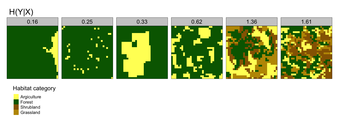
Figure 2.2: Conditional Entropy
- Joint Entropy, H(X,Y) - this provides a measure of the uncertainty in determining the habitat category of a focus cell and an adjacent cell. So landscapes with high H(X,Y) are typically spatially complex with many different habitat types. Note that joint entropy is not capable of distinguishing between patterns that have high spatial aggregation. The variation can be seen in Figure 2.3 .

Figure 2.3: Joint Entropy
- Relative mutual information, U - quantifies the degree of aggregation (clumpliness) of spatial habitat categories from fragmented patterns (lower U) to consolidated patterns (higher U). A landscape comprising a loch within a forest would have a relatively high U, whilst a landscape comprising many different crop types spread across many small fields would have low U. Figure 2.4 gives a mutual entropy landscape
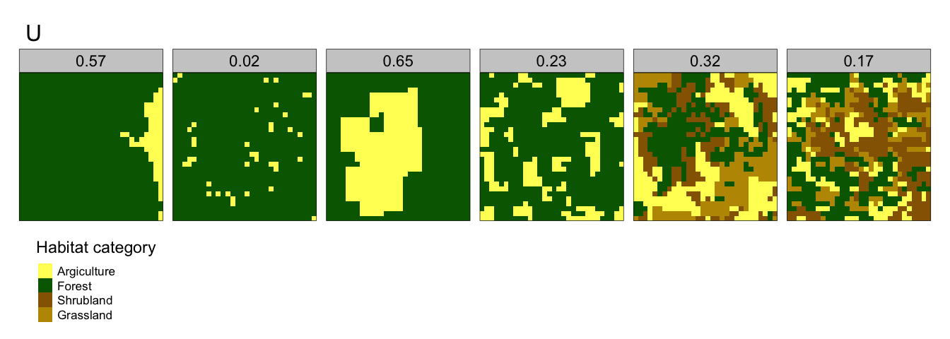
Figure 2.4: Relative Mututal Entropy
2.10 Wader population abundance modelling
Given the set of environmental covariates for each Shetland BBS 1km\(^2\) square and the associated count data for those squares that were surveyed, a machine learning approach using the tidymodels (Kuhn and Wickham 2020) package was taken to fit a random forest regression model (Andy Liaw and Matthew Wiener 2002).
In order to fit the model the count data for each species were adjusted according to their mean detectability. All count data for a given Shetland BBS 1km square was joined with the associated environmental covariate data. The data were then pre-processed so that covariates that have 80% absolute correlations with other covariates are removed; this ensures that possible adverse outcomes due to co-linearity are minimised (Zuur, Ieno, and Elphick 2010). The covariate data within the training dataset were then normalised to a mean of zero and a standard deviation of one. The joined data were then split such that 60% of all data were allocated to model training and the remaining 30% to model testing. A random forest machine learning package (Wright and Ziegler 2017) was used to fit a regression model. 10-fold cross validation was used to resample the data in order to ensure any bias in Shetland BBS survey squares was minimised. Hyper-parameters used to fit the random forest model were selected using a grid containing 10 random variations for each hyperparameter:
min_n- the minimum number of data points in a node that are required for the node to be split furthertrees- the number of trees contained in the ensemblemtry- the number of predictors (covariates) that will be randomly sampled at each split when creating the tree models.
A model was fitted for each combination of hyper-parameters, for each species; giving 50 different models in total. The best model fit for each each species was selected according to the lowest root mean squared error (rmse). The hyper-parameters associated with each best fit were then used to further tune the model for a final fit. The rmse for the final fit was then evaluated against the test dataset, for each species. This gave an abundance estimate (per BBS km\(^2^\)) for each breeding wader species, for each survey year. Summing the density estimate across all squares, by species per year gives an annual mean population estimate for each breeding wader species across all of Shetland, from the 2002 to 2019. Using bootstrap aggregation or bagging, it was possible to generate a lower and upper confidence interval for each of the annual population estimates.
2.11 Lapwing population association with reseeded grassland
Given the population abundance estimate method as outlined in Table 2.10, a specific association between the Lapwing population trend over time and agricultural census data (Scottish Government 2003) was investigated. Specifically the size of different types of annual grassland holdings in Shetland were used as covariate in a regression analysis between 2002 and 2017. The data were tested for normality and it was found that they were log-normally distributed. A generalised additive model for location scale and shape was used to fit the response variable, Lapwing population estimates, against the size of various grassland holdings.
2.12 Wader spatial desnity modelling
Having generated an density estiamtion for each Shetland BBS square, the spatial density can be plotted using the spatial coordinates for each SBBS square, and for each year. Spatial density were generated for each species for 2019 in order to visualise spatial abundance distribution. The net change between the two periods was also plotted so as to visualise the areas of Shetland that have seen a net change in species density between 2002 and 2019.