1 Introduction

The Global Biodiversity Information Facility (GBIF) allows scientists to record and share species occurence information from around the world. Four our study here we will download all occurence records based on the following criteria:

within the administrative boundaries of Oxford City
all records between 2014 to 2019
all human observtions (not museum specimens)
three taxa from the classes Aves, Mammalisa and Insecta

It is likely that the GBIF data will exhibit sampling bias in a number of ways. In general, people are more interested in birds than plants!

# Load libraries
library(tidyverse)
library(rgbif)
library(sf)
library(osmdata)
library(reshape2)

# Clear environment
rm(list = ls())

2 Oxford City study area

First we need to obtain a shapefile for Oxford City, our study area. We can use osmdata from the Open Streetmap foundation to achieve this.

# Get bounding box for Oxford
bb <- getbb('Oxford, U.K.')
# Query OSM for sf data
q <- opq(bbox = bb) %>%
  add_osm_feature(key = 'boundary', value = 'administrative') %>%
  osmdata_sf()

# Convert Oxford polygon to WKT text so that we can query GBIF
ox_WKT <- st_as_text(q$osm_multipolygons$geometry[q$osm_multipolygons$name=="Oxford"])

2.1 Accessing GBIF data

Now we have our spatial query set-up we can query GBIF.

# Setup taxon search keys
# Aves: classKey = 212
# Mammalia: classKey = 359
# Insecta: classKey = 216

classKey <- c(212,359,216)

# Query Oxford species groups
ox_sp <- map(
  .x = classKey,
  ~ occ_search(geometry = ox_WKT, 
                    geom_big = "bbox",
                    classKey = .x,
                    basisOfRecord = 'HUMAN_OBSERVATION',
                    year = '2014, 2019',
                    limit = 10000,
                    hasCoordinate=TRUE,
                    fields = c("scientificName", "speciesKey", "year","decimalLatitude","decimalLongitude", "classKey" ))) %>%
  rbind()

2.2 GBIF results

Now we can manipulate the query from GBIF into a data structure useful for subsequent processing. We have three groups of data in the GBIF object ox_sp, each is grouped by classKey.

# Combine retuned GBIF list queries into a single dataframe 
oxf_sp_df <- ox_sp %>% map_df( ~pluck(.x, "data"))

# Let's look at the data
head(oxf_sp_df)

## # A tibble: 6 x 6
##   classKey speciesKey scientificName decimalLongitude decimalLatitude  year
##      <int>      <int> <chr>                     <dbl>           <dbl> <int>
## 1      212    2490719 Turdus merula…            -1.25            51.8  2019
## 2      212    2492462 Erithacus rub…            -1.25            51.8  2019
## 3      212    2487603 Certhia famil…            -1.26            51.8  2019
## 4      212    5231763 Prunella modu…            -1.25            51.8  2019
## 5      212    5229493 Garrulus glan…            -1.25            51.8  2019
## 6      212    2475532 Alcedo atthis…            -1.24            51.8  2019

#How many observations do we have per taxa?
oxf_sp_df %>% count(classKey)

## # A tibble: 3 x 2
##   classKey     n
##      <int> <int>
## 1      212  9481
## 2      216   806
## 3      359   313

3 Spatial Grid

We need to generate a grid over the Oxford survey area. This will be used to calculate a biodiversity index for each cell within the grid.

# Create a 
ox_poly <- st_as_sf(q$osm_multipolygons %>% filter(name=="Oxford")) %>%
  # Transform coordinates to planar
  st_transform(27700)

# Make a grid of Oxford city
grid_sf <- st_make_grid(
  # Oxford City boundary
  ox_poly, 
  # Cell width in m
  cellsize = 400, 
  # Cells are hexagons
  square = F)

# Plot it
plot(grid_sf, main = "400m wide grid cells covering Oxford City")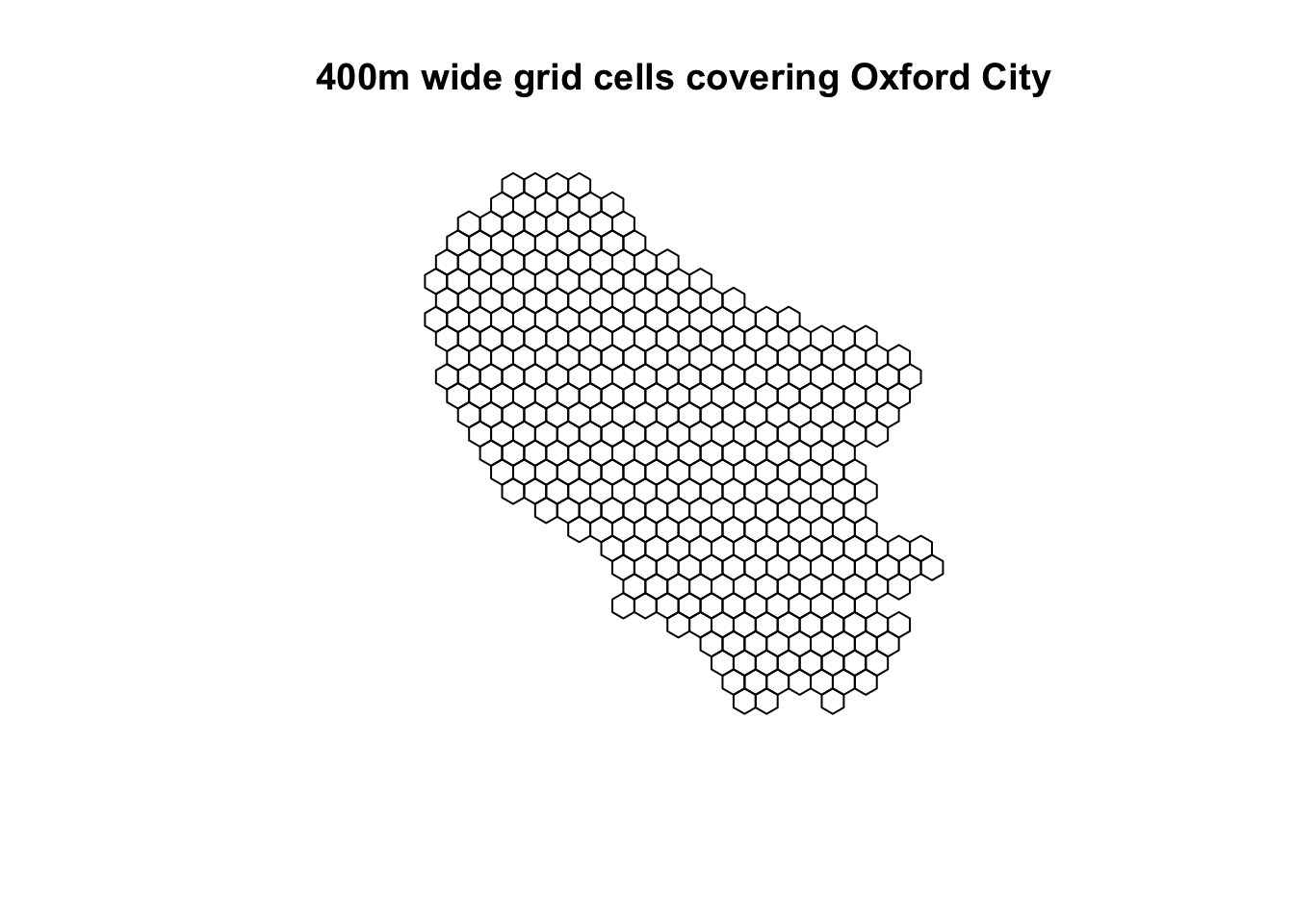

4 Spatial Analysis

Now let’s map species locations to a grid cell.

# Creat sf locatons for species locations in GBIF object 
ox_sp_sf <- oxf_sp_df %>% st_as_sf(coords=c("decimalLongitude","decimalLatitude"),
                                    # Set crs to WGS84
                                    crs = 4326) %>%
  # Reproject to plannar coordinates
  st_transform(27700)

# Add a cell id to the Oxford grid
grid_sf <- grid_sf %>%
  st_sf() %>%
  mutate(cell_id = row_number())

# Generate intersection
intersect <- st_intersects(
  # sf list of species occurences
  ox_sp_sf, 
  # sf grid of Oxford
  grid_sf, 
  # map points to gridcell
  prepared = T) %>%
  # return dataframe
  as.data.frame()

# update column names
names(intersect) <- c("spec_no", "cell_id")

# Create a single table mapping species occurences to cells
grid_species_df <- ox_sp_sf %>% 
  # Create dataframe from result
  as.data.frame %>% 
  # Join with grid/coordinate intersection
  cbind(intersect) %>% 
  # We don't need column spec_no
  dplyr::select(-spec_no) %>%
  # Group and arrange by grid cell ID
  group_by(cell_id) %>%
  arrange(cell_id)

# Plot histogram for each taxa
grid_species_df %>% 
  # Count by cell_id
  ggplot(aes(x=cell_id)) + 
  # Set histogram bin size
  geom_histogram(binwidth=10) + 
  # More Aves taxa records
  facet_wrap(~classKey, scales = "free_y") +
  ggtitle("Histogram of grid cells, by taxa (different y scales)") +
  theme_bw()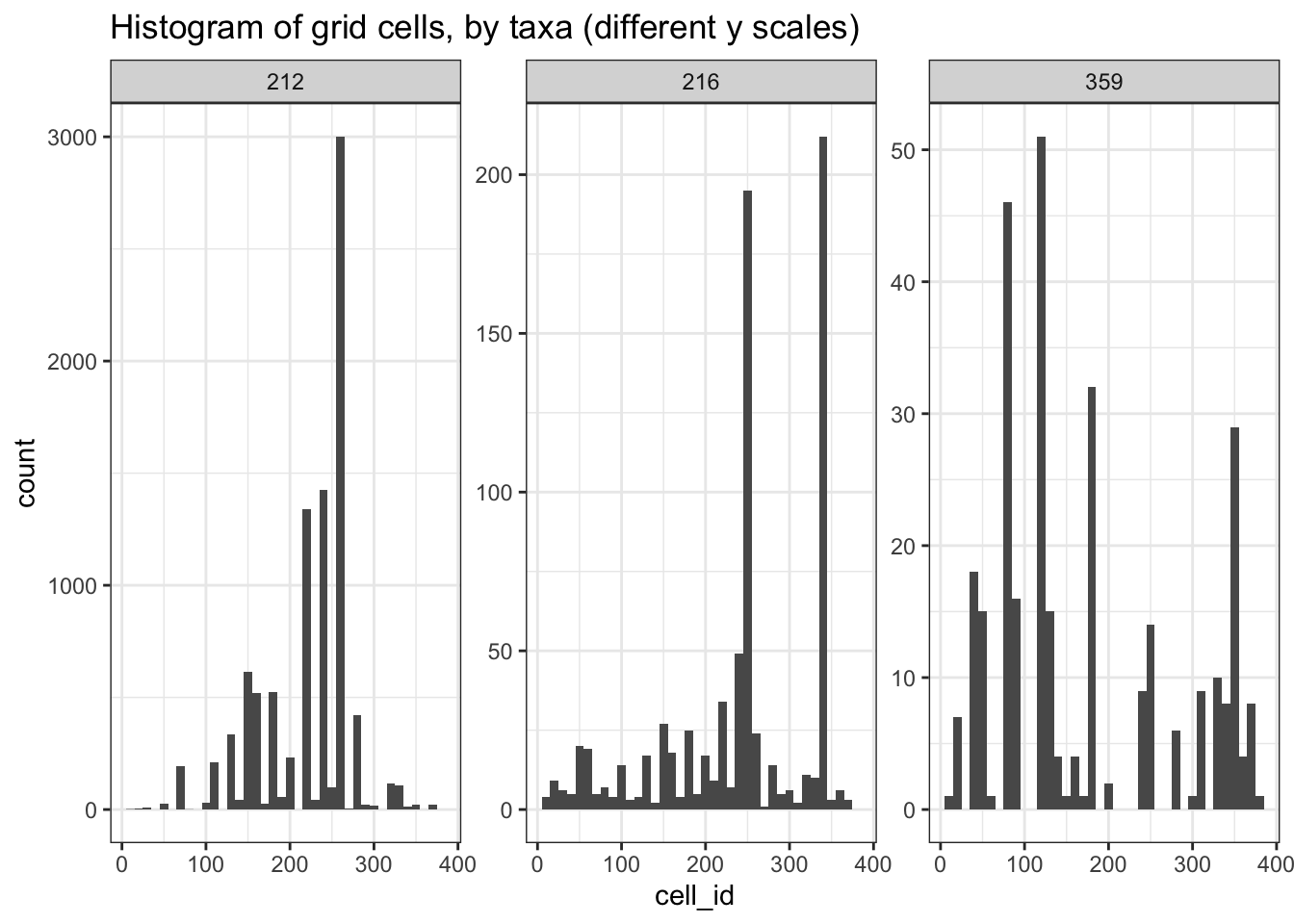

5 Spatial Biodiversity

For each taxa, Calculate the Shannon index for each grid cell

# Load vegan to generate shannon index
library(vegan)


# Function to count the number of species for each grid cell
n_species_cell <- function(df) {
  
  df %>% 
  group_by(cell_id,speciesKey) %>% 
  # Count a given species within a cell
  tally() %>%
  # We need to ungroup to complete
  ungroup() %>%
  # For cells with now species, fill with zeros
  complete(cell_id = 1:nrow(grid_sf), fill=list(n=0))
}

# Count species count grid for each taxa
results <-grid_species_df %>% 
  # Nest by class key
  nest(-classKey) %>%
  # Calculate count by speces and store in separate column
  mutate(n_species_cell = map(data, ~n_species_cell(.x)))

# Function to Create a table of cells by species occurence counts
cell_diversity <- function(df) 
  df %>% 
  pivot_wider(
    id_cols = c("cell_id", "speciesKey"),
    names_from = speciesKey, 
    values_from = n, 
    values_fill = list(n=0)) %>%
  # We can remove cell_id once we have a complete table
  dplyr::select(-cell_id) %>%
  # Calculate shannon diversity for each cell
  diversity("shannon") %>% as.data.frame()

# Calculate shannon diversity in each cell per taxa
results <- results %>%
  mutate(cell_diversity = map(n_species_cell, ~cell_diversity(.x)))

# Add cell shannon diversity to the grid cell sfc
out <- results %>% 
  pluck("cell_diversity") %>% 
  as.data.frame()

# Name the columns  with their classKey
names(out) <- c("Insecta", "Mammalia", "Aves")

# melt data to create one spatial dataset for diversity by grid cell
diversity_grid_sf <- out %>% 
  # Add cell_is as index
  mutate(cell_id = row_number()) %>%
  # melt data with cell_id as index var
  melt(id.vars = "cell_id", measure.vars = c("Insecta","Mammalia","Aves")) %>%
  # join with sf grid polygons
  full_join(grid_sf) %>%
  # Convert dataframe to simple feature collection for plotting
  st_as_sf()

6 Plot Results

We can add a Google background map of Oxford to see where the biodiversity hotspots are.

library(ggmap)
register_google(key="****", write = T)
ox_basemap <- get_map(bb)

ox_basemap <- readRDS("oxford_basemap")

Now we have a Google basemap, let’s visualise this.

library(ggmap)
library(viridis)

# Create map objects and nest in data frame  
diversity_grid_sf <- diversity_grid_sf %>% 
  nest(-variable) %>%
  mutate(plot = map2(data, 
                     variable, 
                     ~ ggmap(ox_basemap) +
                       # Overlay grid data
                       geom_sf(data = .x, 
                       # Fill with Shannon index for each grid cell         
                       aes(fill=value, geometry = geometry), 
                       inherit.aes = F,
                       alpha = 0.5) +
                       # Title of plot
                       ggtitle(.y) +
                       scale_fill_viridis() +
                       # Convert grid data to WGS84
                       coord_sf(crs=st_crs(4326))))

# Now plots and data are nicely stored together
head(diversity_grid_sf)

## # A tibble: 3 x 3
##   variable data               plot  
##   <fct>    <list>             <list>
## 1 Insecta  <tibble [378 × 3]> <gg>  
## 2 Mammalia <tibble [378 × 3]> <gg>  
## 3 Aves     <tibble [378 × 3]> <gg>

# Plot the results
print(diversity_grid_sf$plot)

## [[1]]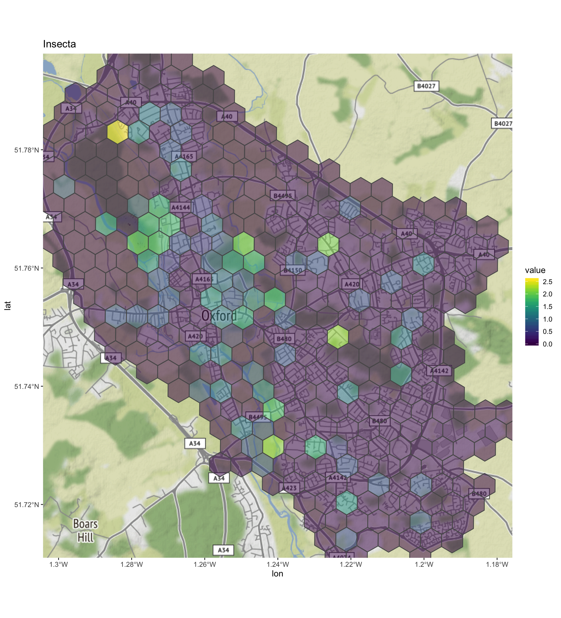

## 
## [[2]]

## 
## [[3]]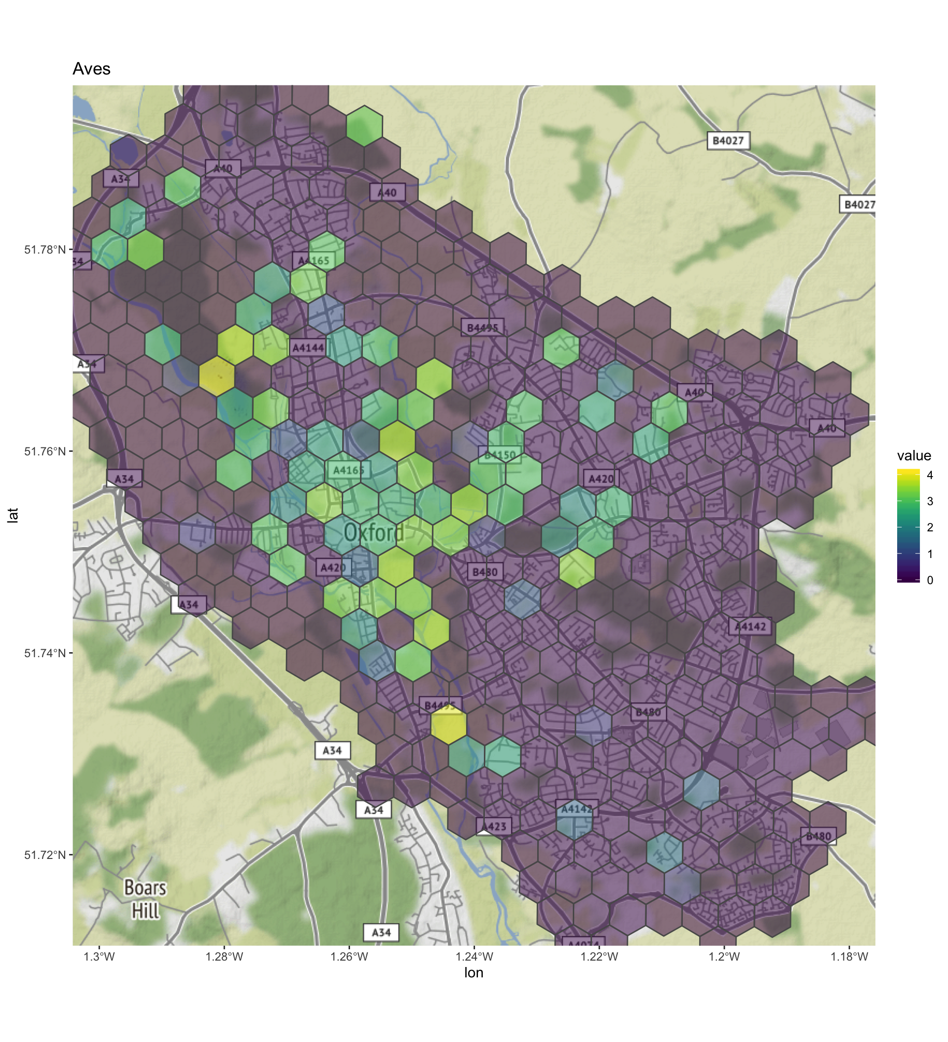

7 Discussion

We can see some interesting results here. As this is not a controlled and randomised set of data, clearly there is significant sampling bias. That being the case, each taxa class clearly show some interesting results when the spatial Shannon diversity is plotted as above:

Insecta - there seems to be a hotspot in the north of Port Meadow. Presumably as this is an ancient wet meadow without any significant human development there maybe noticeable insect diversity here. We can see from the map that most sampling has not been within built up areas.
Mammalia - it seems there are two biodiversity hotspots for mammals in the data analysed. One at the eastern end of Oxford golf course, and the second along Mesopotamia way that runs along the River Cherwell.
Aves - this class had by far the largets number of records, and shows a relatively high density in the centre of the city. There is a diversity hot spot next to the Thames on Port Meadow and alos an area near Ifley Meadows (a local nature reserve). As these are both sites with the Thames running through them, the higher diversity could be due to the inclusion of water fowl?

Biodiversity Mapping