1 Introduction

The GLM relates the mean of the response variable to a linear combination of covariates. The response variable is assumed to be conditionally distributed according to a distribution within the exponential family (bionomial, poisson, gamma etc). The Generalised Additive Model (GAM) is a popular ecology modelling approach, that relaxes the need for the response variable to be characterised by a particular distribution, and instead allows the the relationship between response variable and covariats to be described by the linear combination of smooth curves. GAMs are of the form:

\[\mathop{\mathbb{E}}(Y) = g^{-1} \left( \beta_0 + \sum^J_{j=1}f_j(x_j) \right) \] where:

\(\mathop{\mathbb{E}}\) is the expected value of the response variable, \(Y\),
\(g\) is the link function
\(f_j\) is the smooth function of covariate \(x_j\)
\(\beta_0\) is the intercept.

The smooth functions are the workhorse of the GAM, and are typically spline functions. There are many other forms, depending on the form of the covariate.

1.1 The Northern Gannet Morus bassanus

This vignette makes use of data collected by Camphuysen (2011) ¹, who undertook a survey of the feeding range of Gannet nesting on Bass Rock, a seabird colony in the Firth of Forth. Data were recorded from onboard fishery research vessels in June and July, from 1991 to 2004. Gannet counts were undertaken when the survey ship was fishing. A total of 9,972 km\(^2\) were surveyed, travelling a distance of 33,601 km, and 44,818 Gannets were observed during these surveys. A correction factor for detectability was not applied, with the assumption that all individual Gannets, either swimming or in flight, were detected within a 300m wide strip transect (counts were discontinued in rough conditions, e.g. above wind force 6 on the Beaufort scale).

The research question was to determine when and where gannet feed in the vicinity of the Bass Rock colony. We will use a GAM in an attempt to answer this question, and the approach adopted makes extensive reference to Zuur (2012) ².

# Clear all
rm(list = ls())  

# Load relevant libraries
library(tidyverse)
# Data analysis library
library(skimr)
# GAM modelling
library(mgcv)
# Spatial features library
library(sf)
# Date time manipulation
library(lubridate)
# colourblind-friendly colourschemes
library(viridis)

2 The data

Let’s load the survey data and take a quick peak at its format and structure:

# Read tab delimited file
gannets <- read.table("data_analysis_files/Gannets2.txt", sep = "\t", header = TRUE)
skim(gannets)

Data summary
Name	gannets
Number of rows	12842
Number of columns	14
_______________________
Column type frequency:
numeric	14
________________________
Group variables	None

Variable type: numeric

skim_variable	complete_rate	mean	sd	p0	p25	p50	p75	p100	hist
ID	1	6421.50	3707.31	1.00	3211.25	6421.50	9631.75	12842.00	▇▇▇▇▇
Poskey	1	156209631.43	39586900.46	20015185.00	170001781.25	170007814.50	170011429.75	170015724.00	▁▁▁▁▇
Day	1	12.06	7.18	1.00	7.00	11.00	16.00	30.00	▆▇▇▂▂
Month	1	6.77	0.42	6.00	7.00	7.00	7.00	7.00	▂▁▁▁▇
Year	1	1999.63	4.09	1991.00	1997.00	2001.00	2003.00	2004.00	▂▁▃▂▇
Hours	1	11.03	4.45	2.00	7.00	11.00	15.00	20.00	▅▇▆▇▅
Minutes	1	27.67	17.31	0.00	12.00	28.00	42.00	59.00	▇▆▇▆▆
Latitude	1	56.77	1.08	54.01	56.03	56.66	57.67	59.00	▁▅▇▅▃
Longitude	1	-0.30	1.28	-3.00	-1.39	-0.39	0.79	2.00	▂▇▆▆▆
Area_surveyedkm2	1	0.78	0.34	0.00	0.48	0.66	1.11	2.79	▇▇▅▁▁
Seastate	1	2.93	1.52	0.00	2.00	3.00	4.00	6.00	▆▆▇▇▅
Gannets_in_transect	1	0.67	5.06	0.00	0.00	0.00	0.00	333.00	▇▁▁▁▁
X	1	298511.27	77591.61	127832.60	231037.28	292333.01	365528.92	440991.01	▂▇▆▆▆
Y	1	6297607.44	120950.25	5985125.19	6218768.16	6282868.94	6396381.12	6552041.75	▁▅▇▅▃

We can see that there are no missing data, and that Gannets_in_transect looks like the response variable. Each record represents the number of gannets observed in a transect, and with Area_survyedkm2 we know the number of gannet per km2. If each strip transect is 300m wide, we can establish the transect length if needed.

3 Data analysis

Before we proceed with modelling, let’s do some basic data analysis to make sure everything is in order.

3.1 Visualisng transects

In order to see if the area sampled by year is the same, we can plot the transects by year:

gannets %>%
  # Create an sf geometry for each record
  st_as_sf(coords = c("Latitude","Longitude"), remove = F) %>% 
  # Transform the cooridante reference scheme to planar coordinates 27700 (UK)
  st_set_crs(27700) %>%
  # Plot data
  ggplot() +
  geom_sf(stat="sf", colour= "red", alpha = 0.6, size = 1) +
  # Repeat for each year
  facet_wrap(~Year, ncol = 3) +
  theme_bw() +
  ggtitle("Transects by year")

Looks as if survey effort is fairly consistent, year on year, but on inspecting the data it looks like the area of individual transects are differen, due to differing transect lengths.

# Plot histogra of transect lengths
gannets %>%
  ggplot(aes(x = Area_surveyedkm2)) +
  # Plot histogram of Area_surveyedkm2
  geom_histogram(fill="blue", stat = "count") +
  theme_bw() +
  ggtitle("Histogram of transect area")

We can see that the transect effort, represented by Area-surveyedkm2 is highly variable. This means that we have a variable sampling effort between transects. To account for this variable effect we can use Area-surveyedkm2 as an offset variable. Efecctively this means that if the sampling effort doubles, the number of gannets also doubles.

Also we have some transects where Area-surveyedkm2 is equal to zero. We will remove these, as the boat was not moving and so a transect was not traveresed. We can also add date and time information, and convert coordinates to km (from meters).

# Add extra data items in preparation for modelling
gannets <- gannets %>% 
  # Remove all transects that were equal to zero size
  filter(Area_surveyedkm2 > 0) %>%
  # Create additional data for downstream analysis
  mutate(
    # Create offset variable to compensate for sampling effort
    LArea = log(Area_surveyedkm2),
    # Create continuous time measured in hours
    TimeH = Hours + Minutes/60,
    # Generate a date for each observation
    Date = dmy(sprintf('%02d%02d%04d', Day, Month, Year)),
    # Generate day in year
    DayInYear = yday(Date),
    # Change X and Y into km
    Xkm = X/1000,
    Ykm = Y/1000
         )

4 Gannet density in space and time

We can now undertake some further data exploration and look at how surveyed Gannet density varies in space and time. The first plot below shows how observed gannet density varies by year - the bigger the red dot, the larger the density of Gannet recorded.

# First calculate gannet density per transect
gannets <- gannets %>%
  mutate(gannet_density = Gannets_in_transect/Area_surveyedkm2)

# Plot gannet density in space by year
gannets %>%
  ggplot() +
  geom_point(
    # Convert m to km for transect locations
    # Make each dot size equal to gannet abundance
    aes(x = Xkm, y = Ykm, size = gannet_density), 
    colour = "red",
    alpha = 0.6
    ) +
  # Project coordinates to plananr
  coord_sf(crs = 27700) +
  facet_wrap(~Year, ncol = 3) +
  # Add a scale for the size of each dot
  scale_size(range = c(0, 10)) +
  labs( x = "Latitude", y = "Longitude") +
  theme_bw() +
  ggtitle("Spatial Gannet density by year")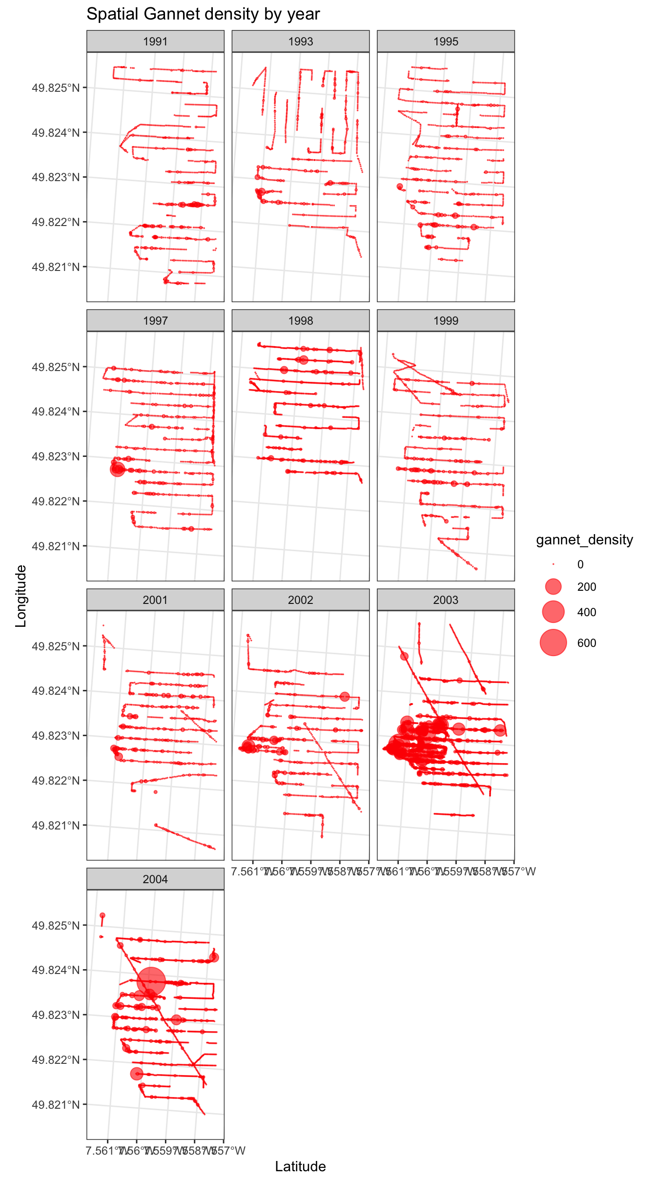

This clearly shows us that gannet density changes in space year on year, indicating that a three dimenstional GAM smooth of the form \(f(Year_i, lat_i, long_i)\) is required to capture this effect.

What can we tell about the distribution of gannet density?

gannets %>%
  ggplot(aes(x = gannet_density)) +
  # Plot histogram of Area_surveyedkm2
  geom_histogram(fill="blue", bins = 30) +
  theme_bw() +
  ggtitle("Histogram of observed Gannet density")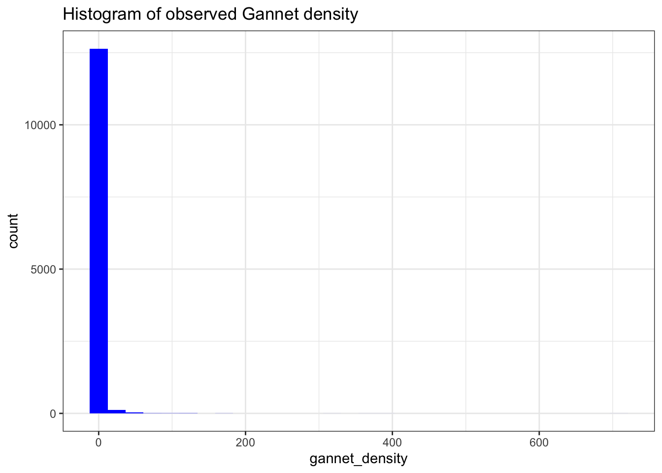

We can see that the data is clearly zero-inflated. The vast majority of observations are zero. But the data are highly dispersed too, as there are density observations of 600.

We can also observe gannet density by hour of day, for each year:

# Plot gannet density by day and hour
gannets %>%
  ggplot() +
  geom_point(
    # Convert m to km for transect locations
    # Make each dot size equal to gannet abundance
    aes(x = TimeH, y = DayInYear, size = gannet_density), 
    colour = "blue",
    alpha = 0.5
    ) +
  facet_wrap(~Year, ncol = 3) +
  labs( x = "Hour of day", y = "Day in Year") +
  theme_bw() +
  ggtitle("Gannet density by day of year and hour of day, for each year")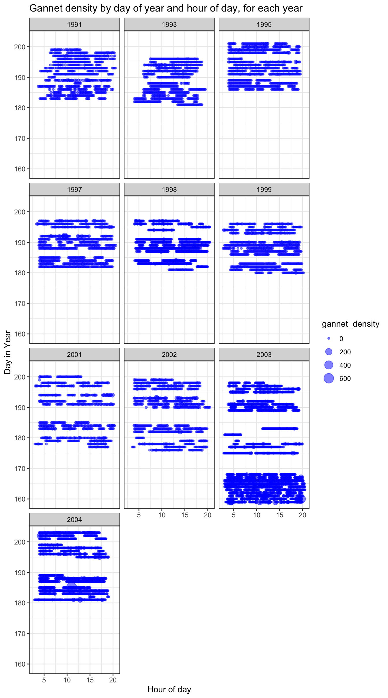

We can see that in 2003 surveying started earlier in the year.

5 Gannet abundance GAM

We would like to build a model to predict gannet abundance across time and space. Our initial data exploration has shown that gannet abundance varies in a non-linear fashion across days, months and years. Below we will iteratively build up a model and each step attempt to evaluate the overall model fit.

5.1 A year effect and offset variable

# Create first gam for gannet abundance
m1 <- gam(
  # Set the model equation: abundnce is driven by a smooth of year plus 
  # an offset equal to the log of the sample area
  Gannets_in_transect ~ s(Year) + offset(LArea), 
  # We assume that gannet abundance (a count) is from a poisson distribution
  family = poisson, 
  data = gannets)

# Show summary of model fit
summary(m1)

## 
## Family: poisson 
## Link function: log 
## 
## Formula:
## Gannets_in_transect ~ s(Year) + offset(LArea)
## 
## Parametric coefficients:
##             Estimate Std. Error z value Pr(>|z|)    
## (Intercept) -0.16845    0.01212   -13.9   <2e-16 ***
## ---
## Signif. codes:  0 '***' 0.001 '**' 0.01 '*' 0.05 '.' 0.1 ' ' 1
## 
## Approximate significance of smooth terms:
##           edf Ref.df Chi.sq p-value    
## s(Year) 8.886  8.995   3093  <2e-16 ***
## ---
## Signif. codes:  0 '***' 0.001 '**' 0.01 '*' 0.05 '.' 0.1 ' ' 1
## 
## R-sq.(adj) =  0.000322   Deviance explained = 6.73%
## UBRE = 2.4997  Scale est. = 1         n = 12820

The results show that the smooth of year is significant in the model, and that the smooth has 8.9 effective degrees of freedom. We can plot the effect of the smooth by year as follows:

plot(m1)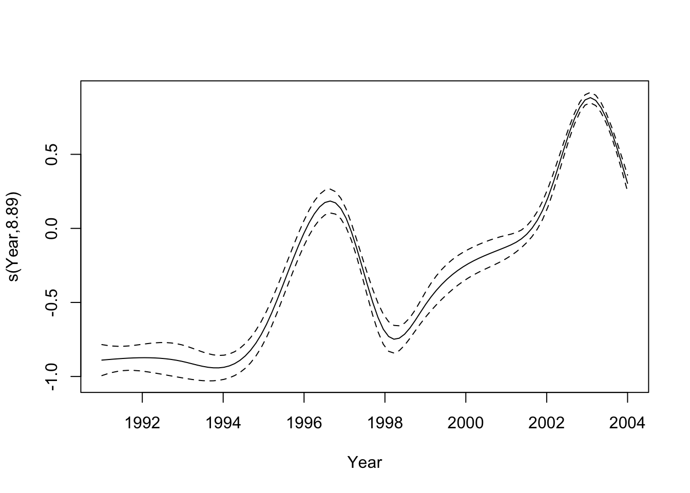

We can see that the effect of the Year variable increases to 1997, drops significantly in 1998 and then increases again in 2003. This is consistent with the chart above. To calulcate the degree of overdispersion we look at the residual errors as follows:

# Overdispersion is calculated as the sum of squared Pearson residuals divided by 
# sample size minus the number of parameters 
overdispersion <- function(m){
  err <- resid(m, type = "pearson")
  overdispersion <- sum(err^2)/m$df.residual
  return(overdispersion)
}

overdispersion(m1)

## [1] 36.92865

There is considerable overdisperson in this first model. The summary for m1 shows that the \(R^2\) is very low too.

5.2 Additional covariates

From our initial data exploration we noted a number of apparent effects from the data. We can now add the effect of the geographical location of the surveying via a two-dimensional smooth. As the locational covariates are at a very different scale and units to the other covariates (all time based) we use the te or tensor product smoother. From our data exploration work, we also noted that a three dimensional function of the form \(f(Year_i, lat_i, long_i)\) might be significant. Finally we can also include the sea state as a categorical variable, and the second combinatory effect of time of day coupled with day of the year (which we model as a tensor product).

# Create first gam for gannet abundance
m2 <- gam(
  # Set abundance as ther respone variable:
  Gannets_in_transect ~ 
    # 1 - TE smooth of time of day combined with day of year
    te(TimeH, DayInYear) + 
    # 2 - seastate as a categorical variable
    as.factor(Seastate) +
    # 3 - An offset equal to the log of the sample area
    offset(LArea) +
    # 4 - TE smooth of lat, long and year 
    te(Xkm, Ykm, Year),
  # We assume that gannet abundance (a count) is from a poisson distribution
  family = poisson, 
  data = gannets)

# Show summary of model fit
summary(m2)

## 
## Family: poisson 
## Link function: log 
## 
## Formula:
## Gannets_in_transect ~ te(TimeH, DayInYear) + as.factor(Seastate) + 
##     offset(LArea) + te(Xkm, Ykm, Year)
## 
## Parametric coefficients:
##                      Estimate Std. Error z value Pr(>|z|)    
## (Intercept)          -0.62841    0.04602 -13.654  < 2e-16 ***
## as.factor(Seastate)1  0.08529    0.04527   1.884 0.059576 .  
## as.factor(Seastate)2 -0.16130    0.04573  -3.528 0.000419 ***
## as.factor(Seastate)3 -0.26007    0.04679  -5.558 2.73e-08 ***
## as.factor(Seastate)4 -0.37802    0.05179  -7.299 2.90e-13 ***
## as.factor(Seastate)5 -0.17460    0.06644  -2.628 0.008590 ** 
## as.factor(Seastate)6 -0.43253    0.10326  -4.189 2.81e-05 ***
## ---
## Signif. codes:  0 '***' 0.001 '**' 0.01 '*' 0.05 '.' 0.1 ' ' 1
## 
## Approximate significance of smooth terms:
##                       edf Ref.df Chi.sq p-value    
## te(TimeH,DayInYear)  23.9   24.0   1830  <2e-16 ***
## te(Xkm,Ykm,Year)    123.1  123.9   8567  <2e-16 ***
## ---
## Signif. codes:  0 '***' 0.001 '**' 0.01 '*' 0.05 '.' 0.1 ' ' 1
## 
## R-sq.(adj) =  0.0668   Deviance explained = 30.6%
## UBRE = 1.6279  Scale est. = 1         n = 12820

# Calculate overdispersion
overdispersion(m2)

## [1] 12.07295

This makes a significant difference to the overdispersion which has now been reduced to 12. This is still significant, and the lastest term introduced requires 124 degrees of freedom so is computationally expensive. Also the \(R^2\) has improved slightly (though not significantly).

5.3 Negative-binomial GAM

One final thing is to try a negative-binomial distribution in place of the poisson distribution we have used so far. A ngeative binomial can be used to represent non-negative count data. In such a model, the variance can vary independent of the distribution mean and as such might better capture the overdispersion we are seeing.

# Create first gam for gannet abundance
m3 <- gam(
    # Set abundance as ther respone variable:
    Gannets_in_transect ~ 
    # 1 - TE smooth of time of day combined with day of year
    te(TimeH, DayInYear) + 
    # 2 - seastate as a categorical variable
    as.factor(Seastate) +
    # 3 - An offset equal to the log of the sample area
    offset(LArea) +
    # 4 - TE smooth of lat, long and year 
    te(Xkm, Ykm, Year),
  # We assume that gannet abundance (a count) is from a negative-binomial distribution
  # Set theta equal to 0.1
  family = negbin(0.1), 
  link = log,
  data = gannets)

# Show summary of model fit
summary(m3)

## 
## Family: Negative Binomial(0.1) 
## Link function: log 
## 
## Formula:
## Gannets_in_transect ~ te(TimeH, DayInYear) + as.factor(Seastate) + 
##     offset(LArea) + te(Xkm, Ykm, Year)
## 
## Parametric coefficients:
##                      Estimate Std. Error z value Pr(>|z|)    
## (Intercept)          -0.52398    0.12844  -4.080 4.51e-05 ***
## as.factor(Seastate)1  0.21261    0.15648   1.359   0.1742    
## as.factor(Seastate)2 -0.23423    0.14832  -1.579   0.1143    
## as.factor(Seastate)3 -0.16531    0.14498  -1.140   0.2542    
## as.factor(Seastate)4 -0.26461    0.15211  -1.740   0.0819 .  
## as.factor(Seastate)5 -0.04352    0.18410  -0.236   0.8131    
## as.factor(Seastate)6 -0.36137    0.23092  -1.565   0.1176    
## ---
## Signif. codes:  0 '***' 0.001 '**' 0.01 '*' 0.05 '.' 0.1 ' ' 1
## 
## Approximate significance of smooth terms:
##                       edf Ref.df Chi.sq  p-value    
## te(TimeH,DayInYear) 22.24  23.48  69.51 6.27e-06 ***
## te(Xkm,Ykm,Year)    90.42 101.74 708.13  < 2e-16 ***
## ---
## Signif. codes:  0 '***' 0.001 '**' 0.01 '*' 0.05 '.' 0.1 ' ' 1
## 
## R-sq.(adj) =  0.0301   Deviance explained = 27.2%
## UBRE = -0.63999  Scale est. = 1         n = 12820

# Calculate overdispersion
overdispersion(m3)

## [1] 1.430392

This appeared to work well. Our overdispersion measure started at 37 with model 1, and now is at 1.4 with model 3. We can run an anova test to see which smooths are significant within the final model.

anova(m3)

## 
## Family: Negative Binomial(0.1) 
## Link function: log 
## 
## Formula:
## Gannets_in_transect ~ te(TimeH, DayInYear) + as.factor(Seastate) + 
##     offset(LArea) + te(Xkm, Ykm, Year)
## 
## Parametric Terms:
##                     df Chi.sq p-value
## as.factor(Seastate)  6   19.1 0.00399
## 
## Approximate significance of smooth terms:
##                        edf Ref.df Chi.sq  p-value
## te(TimeH,DayInYear)  22.24  23.48  69.51 6.27e-06
## te(Xkm,Ykm,Year)     90.42 101.74 708.13  < 2e-16

The results show that the tensor product multivariate smooths are the most significant in the model. We can visiualise there effect using the vis.gam function:

# Plot X,Y smooth
vis.gam(m3, 
        # Covariates we want to visualise
        view = c("Xkm","Ykm"), 
        # Number of points in either direction for calculating the surface
        n.grid = 50, 
        # Define plot orientation
        theta = 35, phi = 32, 
        # Define labels
        zlab = "smooth", xlab = "Xkm", ylab = "Ykm",
        # Pick colour scheme
        color = "topo", 
        # Give plot a title
        main = " te(Xkm, Ykm)")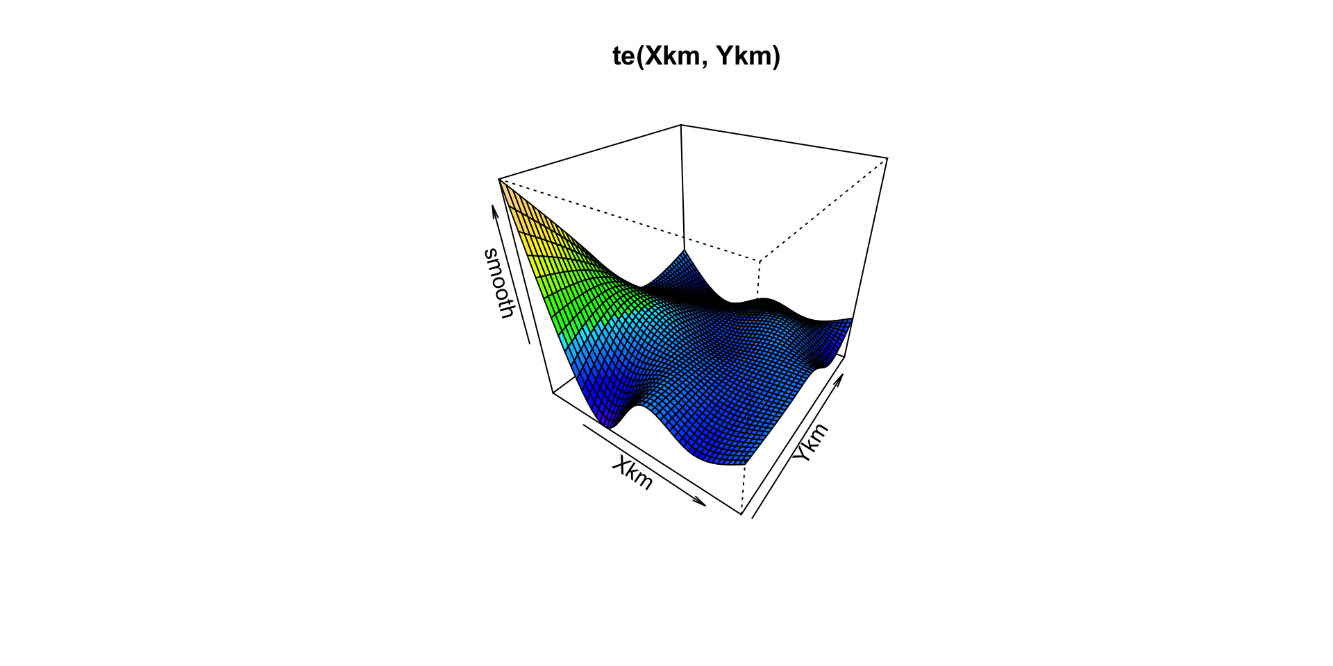

# Plot TimeH,DayInYear smooth
vis.gam(m3, 
        # Covariates we want to visualise
        view = c("TimeH","DayInYear"), 
        # Number of points in either direction for calculating the surface
        n.grid = 50, 
        # Define plot orientation
        theta = 35, phi = 32, 
        # Define labels
        zlab = "smooth", xlab = "TimeH", ylab = "DayInYear",
        # Pick colour scheme
        color = "topo", 
        # Give plot a title
        main = "te(TimeH, DayInYear)")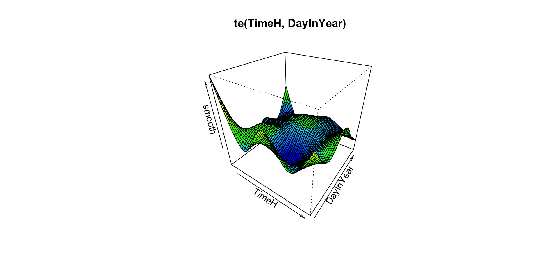

It seems that for the te(X,Y) smooth the response is concentrated towards the south-west of the area. Presumably this is where Gannets spend most of their time foraging. The te(TimeH, DayInYear) smooth is perhaps more difficult to interpret. It appears that the effect on the response variable is more significant at the start of the year, than at the end.

6 Plot a prediction

To map fitted values, we first create a data.frame of covariates required by the model. Then we use the predict function to generate a set of values. In the example below we will fit a model to give abundance of gannets within 1km squares. First we need to create the data to use when predicting the overall response. We will make a prediction for middle of the day, half way through 2002.

# Create dataframe containing all data
m3_data <- expand.grid(
  # Create X values for model - one every 1km
  Xkm = X_values <- seq(min(gannets$Xkm), max(gannets$Xkm), by = 1), 
  # Create Y values for model - one every 1km
  Ykm = Y_values <- seq(min(gannets$Ykm), max(gannets$Ykm), by = 1), 
  # Pick a year to model
  Year = 2002,
  # Pick a seastate
  Seastate = as.factor(1),
  # Set offset area equal to cell size (1km)
  LArea = 1,
  # Pick the middle of the year
  DayInYear = 180,
  # Pick middle of the day
  TimeH = 12
)

# Now make a prediction using m3
abundance_pred <- predict(m3, m3_data)
# Add it to the prediction grid
m3_data$Nhat <- abundance_pred

# Now plot
m3_data %>%
  ggplot() +
  geom_tile(aes(x=Xkm, y=Ykm, fill = Nhat, width = 10, height = 10)) +
  coord_equal() +
  labs(fill="Density") +
  scale_fill_distiller(palette = "Spectral") +
  theme_bw() +
  ggtitle("Gannet density estimate, Year=2002, Day=180, TimeH=12")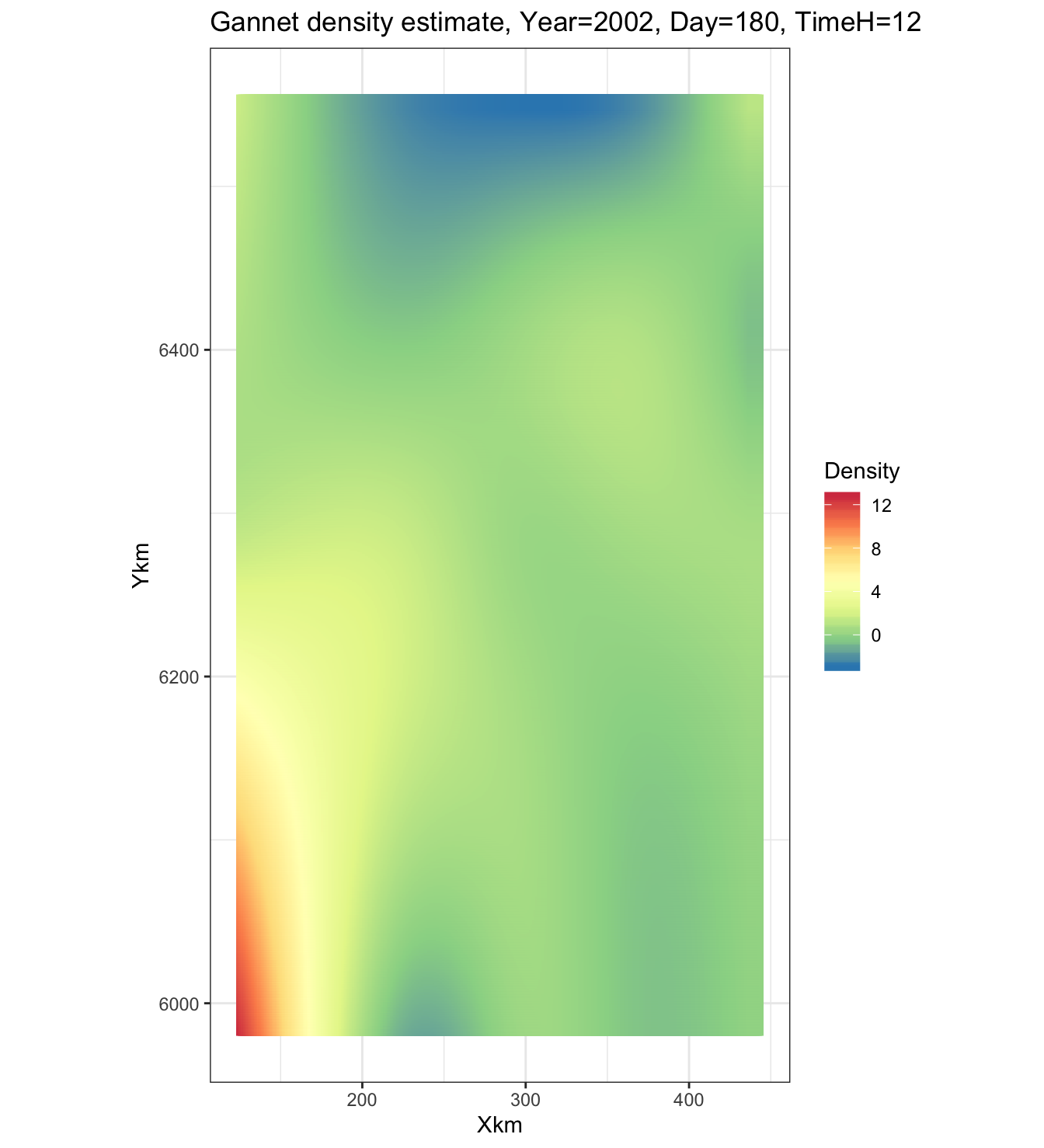

We can see that there is a slight increase in observed gannet density in the south west corner of the map. If we sum every cell in the grid we should get the total Gannet abundance at the time specified above (middle of 2002):

sum(m3_data$Nhat)

## [1] 123167

7 Discussion

GAMs are a powerful technique for fitting enivironmental data that do not fit well with simple linear models. In the example above we took survey data and created a predictive model that enabled us to make an estimate of total Gannet abundance across the entire survey area. As of 2015, the colony size is thought to be around 150,000 birds on Bass Rock³. So the final abundance estimate for 2002, seems consitent with this. Note we did not account for detectability in the above. It was assumed that everything present was observed within the 300m wide transect.

8 References

Northern Gannets in the North Sea, KCJ Camphuysen (2011). https://britishbirds.co.uk/wp-content/uploads/2014/05/V104_N02_P060%E2%80%93076_A.pdf ↩
Beginner’s Guide to Generalized Additive Models with R, Zuur, AF (2012). https://highstat.com/index.php/beginner-s-guide-to-generalized-additive-models-with-r ↩
BBC News (2015), https://www.bbc.co.uk/news/uk-scotland-edinburgh-east-fife-31453488 ↩

Generalised Additive Models