1 Introduction

Geolocation by light allows for tracking animal movements, based on measurements of light intensity over time by a data-logging device; a geolocator. Recent developments of ultra-light devices (<2 g) have broadened the range of target species and boosted the number of studies using geolocators. In this vignette we look at calculating and plotting the migration path of the Red-neck Phallarope Phalaropus lobatus. The use of data was kindly given by Tong Mu from the Department of Ecology and Evolutionary Biology, Princeton University, USA. The original paper defining the tracking method and results can be found here¹. The migration track of Phalarope BA055 starts from the breeding grounds of Chukotka in around the Bering Sea, to the over wintering grounds in the East Indies; a round trip of some 20,000km.

This vignette makes extensive use of the code within the manual Light-Level Geolocator Analyses: A user’s guide ².

# Clear all
rm(list = ls())  

# Load librarieis
library(GeoLocTools)
library(GeoLight)
library(TwGeos)
library(SGAT)
library(MASS)
library(dplyr)
library(raster)
library(maptools)
library(FLightR)
library(ggmap)

The data collected uses a geolocator made by Migrate Technology Ltd logger. The configuration of the geolocator was as follows:

MODE: 3 (full range light, temperature, wet/dry and conductivity recorded)
LIGHT: Sampled every minute with max light recorded every 5mins.
TEMPERATURE: Sampled every 5mins with max and min recorded every 4hrs.
WET/DRY and CONDUCTIVITY: Sampled every 30secs with number of samples wet recorded every hr (capped at 7mins wet per hour), max conductivity recorded every 4hrs.
Max record length = 15 months. Total battery life upto 23 months. Logger is currently 14 months old.
Programmed: 07/07/2016 22:13:14. Start of logging (DD/MM/YYYY HH:MM:SS): 07/07/2016 22:13:14
Age at start of logging (secs): 4488620, approx 2 months
End of logging (DD/MM/YYYY HH:MM:SS): 01/07/2017 08:02:17
Age at end of logging (secs): 35454822, approx 14 months
Timer (DDDDD:HH:MM:SS): 00358:09:43:22
Drift (secs): 341. Memory not full.
Pointers: 64826,123696,3158064,3158064,0,0,61% light mem used,70% wet/dry/temp mem used
Tcals (Ax^3+Bx2+Cx+D): -35407.051,64980.930,-40521.832,8621.896
Approx 0.5’C resolution. Conductivity >63 for ‘wets’ count. Light range 4, ambient. XT.

Let’s load up the raw data from BA055’s journey.

raw <- read.csv("data_analysis_files/geoloc_data/Phalarope.csv")

# Create datasets for geo-location and additional measurements
d.lux <- raw %>% 
  # Select omly data related too light levels
  dplyr::filter(sensor.type == "solar-geolocator-raw")%>%
  # Convert data too POSIX format
  mutate(Date = as.POSIXct(.$Date, tz = "UTC")) %>%
  # Select only only one track (there are two in the file)
  filter(tag.local.identifier == "BA055") %>%
  # Log transfrom light intensity
  mutate(Light = log(.$Light)) %>%
  # Selecy only those columns required
  dplyr::select(Date, Light)

head(d.lux)

##                  Date    Light
## 1 2016-07-08 10:08:14 4.659725
## 2 2016-07-08 10:13:14 4.761849
## 3 2016-07-08 10:18:14 2.692056
## 4 2016-07-08 10:23:14 3.911303
## 5 2016-07-08 10:28:14 2.525008
## 6 2016-07-08 10:33:14 2.324347

We now have the lux information by date and time. Now we need to calibrate the data.

# BA055's departure/capture point
lon.calib <- 177.05
lat.calib <- 62.55

# Calibration times - prior to migration
tm.calib <- as.POSIXct(c("2016-07-08", "2016-07-22"), tz= "UTC")
# Days on track
tm.track <- as.POSIXct(c("2016-07-23", "2017-06-10"), tz= "UTC")

2 Calculating Twilight times

Now we can calculate twilight times.

# Light level threshold between night and day
threshold <- 2
# adjusts the y-axis to put night (dark shades) in the middle
offset <- 4
# maximum light level (log transformed)
lmax <- 12

# Interactive process that cannot be executed in rmarkdown. 
# Can define minimum dark period. Here it is set at 4 hours (240 minutes)

### The function preprocessLight opens two interactive plots and you have to go through 4 different steps: 

### -1. Define the desired period with left click on the left boundary and right clock on the right boundary. Press "a"     
###     to go to the next step. 
### -2. Define seeds (one or multible) - a position during the night that shows clear sunrise/sunset boundaries. You can        
###     click on plot 1 to zoom into a region that will be shown in plot 2 (seeds need to be defined in plot 2). Press 
###     "a" to go to the next step. 
### -3. Add non-defined twilights if necessary. Press "a" to go to the next step. 
### -4. You can go through each twilight using the forward and backward arrows or click on specific twilight times. The 
###     selected twilight times will be shown in the second plot. You can change the twilight time by clickinga at the 
###     desired position and press "a". Press "q" to close plots and return to R.
### See ?preprocessLight for other functions

#twl <- preprocessLight(d.lux, 
#                       threshold, 
#                       offset = offset, 
#                       zlim = c(0, lmax), 
#                       #dark.min = 240,
#                       gr.Device = "x11")

#write.csv(twl,"BA055v2_twl.csv")

# Load BA055 track twilight data
twl <- read.csv("BA055v2_twl.csv")

# Converts twilights into appropriate format
twl$Twilight <- as.POSIXct(strptime(twl$Twilight, format="%Y-%m-%d %H:%M:%S"), tz = "UTC")

# Account for storing maximum values for each 5 minute period. This step will depend on tag type. 
#twl <- twilightAdjust(twl, 150)

# Show results of defining twilights against raw light data
lightImage(d.lux, offset = offset, zlim = c(0,lmax))
tsimagePoints(twl$Twilight, 
              offset = offset, 
              pch = 16, 
              cex = 0.5,
              # Sunrise is blue, sunset is red
              col = ifelse(twl$Rise, "dodgerblue", "firebrick"))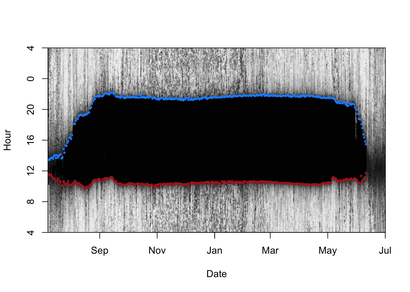

There are some sunrises and sunsets that have been misclassified, so we can use the twlightEdit function to move these to where they should be.

twl <- twilightEdit(twilights = twl,
                    offset = offset,
                    window = 4,           # two days before and two days after
                    outlier.mins = 25,    # difference in mins
                    stationary.mins = 25, # are the other surrounding twilights within 25 mins of one another
                    plot = TRUE)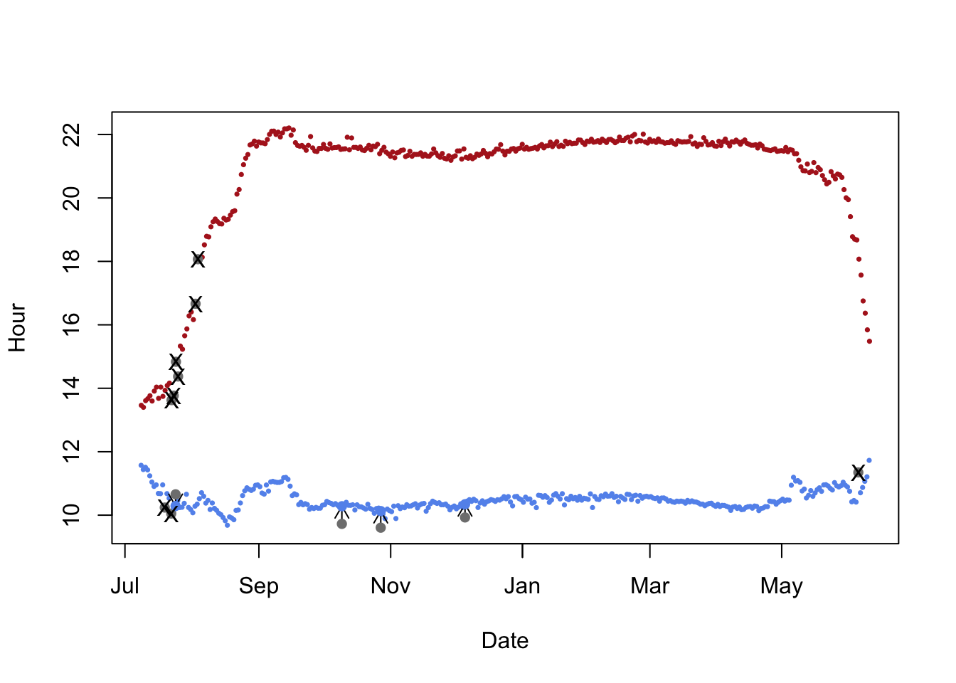

3 Calibration

Geolocators sample light levels at regular intervals and calibration is needed to establish the relationship between the observed and the expected light levels for each device. This relationship is depicted by the calibration parameters (slopes), calculated using the data recorded in known (calibration) geographic positions, e.g. where the animal was tagged, recaptured or observed.

Below we show the recorded light levels upto a yellow vertical dashed line - we use this timeframe for calibrating the geolocator. These are observations after the bird has been tagged but before it has left the tagging location on its annual migration. In theory the bird returned to a similar location for breeding, but the data are not well formed, so we are unable to use this as a second calibration period. This will also mean that the a return flight path cannot be fully calculated. This can be clearly seen on the right hand side of the plot below.

# Subset the twilight data with calibration periods
d.calib <- twl %>%
  # Claibrate using dates before migration
  filter(Twilight >= tm.calib[1]) %>%
  filter(Twilight <= tm.calib[2]) %>%
  # And those dates not removed during pre-porcessing
  filter(!Deleted)

# Let's visualise the calibration dates on the light image
lightImage( tagdata = d.lux,
            offset = offset,     
            zlim = c(0, 8))

# Plot the twilight bands
tsimagePoints(twl$Twilight, offset = offset, pch = 16, cex = 0.5,
              # Sunrise is blue, sunset is red
              col = ifelse(twl$Rise, "dodgerblue", "firebrick"))

# Plot the calibration period between vertical oragne lines
abline(v = tm.calib, lwd = 2, lty = 2, col = "orange")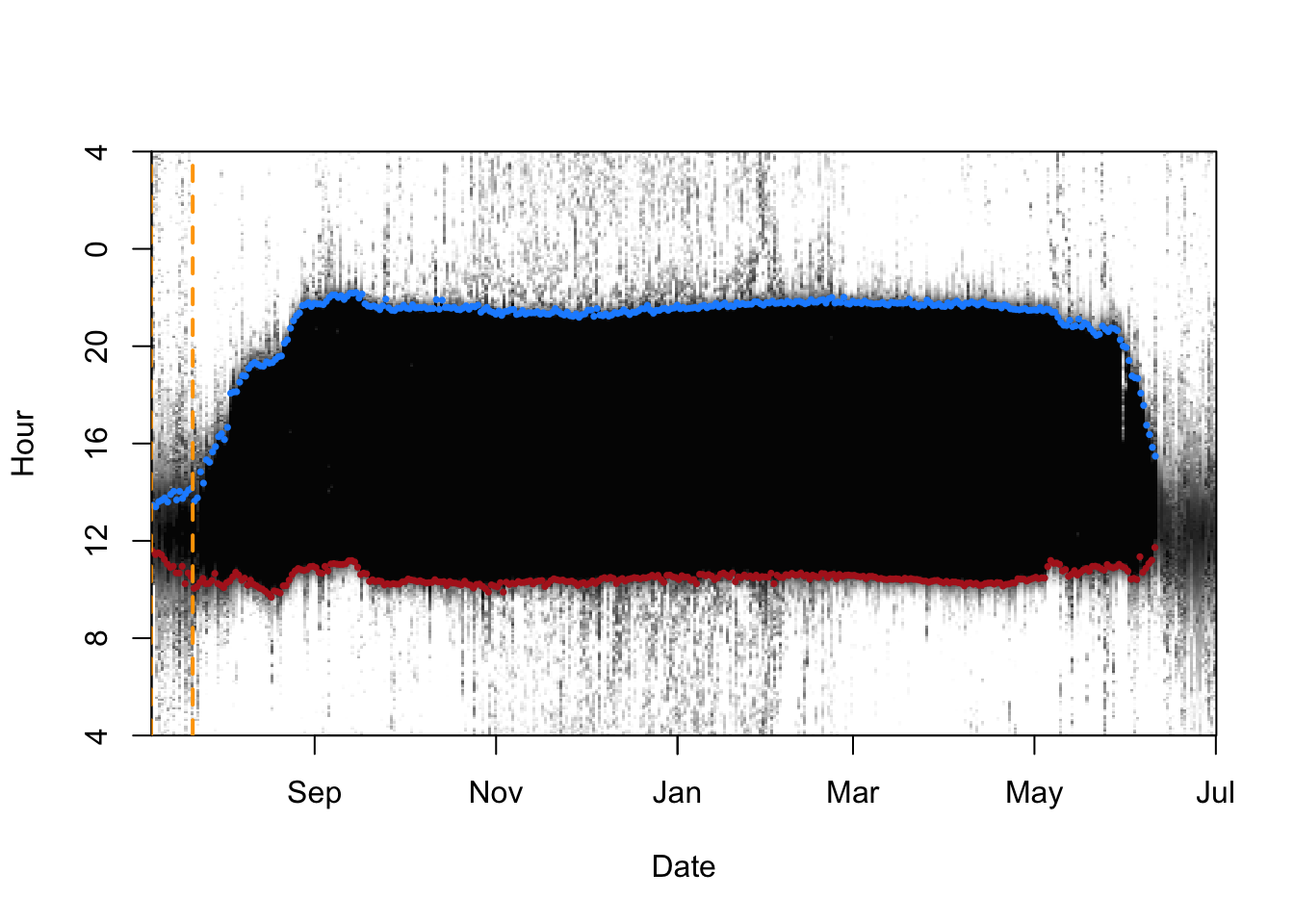

The threshold calibration method is mainly used to derive positions by defining sunrise and sunset times from the light intensity pattern for each recorded day. This method requires calibration: a predefined sun elevation angle for estimating latitude by fitting the recorded day⁄night lengths to theoretical values across latitudes. Therewith, almost constant shading can be corrected for by finding the appropriate sun elevation angle.

3.1 Hills-Ekstrom calibration

There is an alternative approach to calibration using the Hill-Ekstrom³ theory to estimate the sun zenith. This approach proposes that the zenith angle should lead to the lowest variance in latitude estimates (i.e. flattest) during stationary periods. The Hill-Ekstrom calibration is based on an increasing error range in latitudes with an increasing mismatch between light level threshold and the used sun angle. This error is strongly amplified with proximity to the equinox times due to decreasing slope of day length variation with latitude.

# Set dates for calibration to be where the sd is minimised
startDate <- "2016-09-30" #tm.track[1]
endDate   <- "2016-11-30" #tm.track[2]
  
start = min(which(as.Date(twl$Twilight) == startDate))
end = max(which(as.Date(twl$Twilight) == endDate))

zenith_he <- findHEZenith(twl, tol=0.01, range=c(start,end))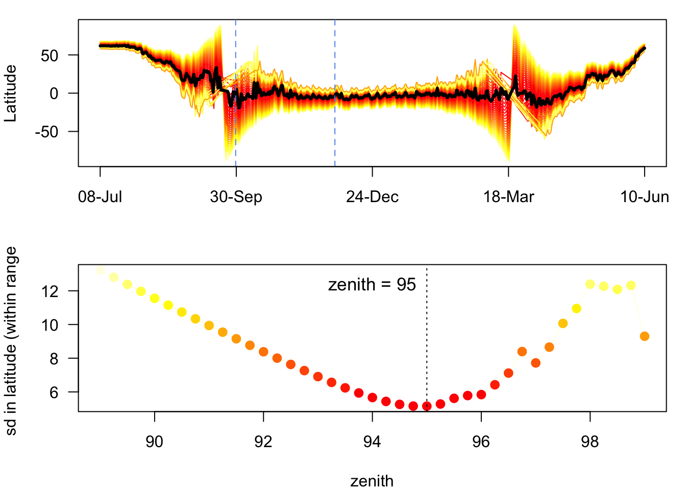

The top panel shows the entire migration path (latitude at each date) using different zenith angles with the black line indicating the latitude estimates with the smallest variation within the specified calibration range (in between the two blue dashed lines). We can see that the standard deviation of the estimate for zenith is minimised at around 94.5 (lower panel).

4 Movement model

We need to provide a mean and standard deviation for a gamma distribution of flight speeds that get applied to each day of the analysis period. We typically want short (near zero) distance daily flights to be common and long distance daily flights to be relatively rare.

# Species movement model
# changed beta to fit slower moving birds
beta  <- c(2.2, 0.06)
matplot(0:100, dgamma(0:100, beta[1], beta[2]),
        type = "l", col = "orange",lty = 1,lwd = 2,ylab = "Density", xlab = "km/h")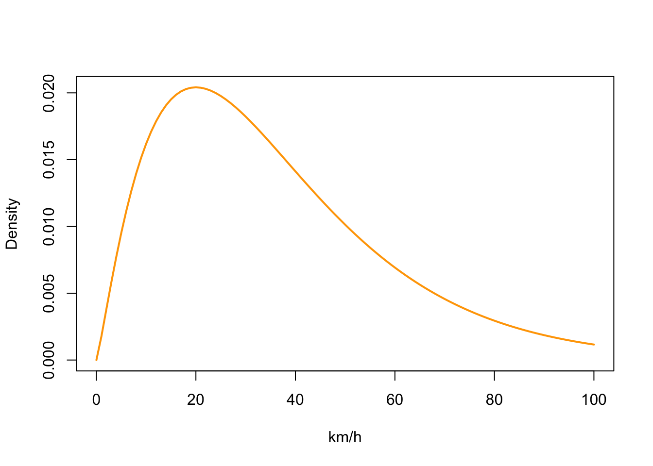

5 Plot initial track

Now we can visualise an initial track for BA055, prior to performing a more sophisticated analysis of the flight path.

#  Creates path from simple threshold estimates. 
# Varying the "tol" value will change the duration of period surrounding the equinoxes that latitudes will not be estimated from light-level 
# data. Instead latitudes will be estimated in a linear progression from the first twilight before the equinox period until the first twilight
# after the equinox ### period
path <- thresholdPath(twl$Twilight, 
                      twl$Rise, 
                      zenith = zenith_he, 
                      tol = 0.1, 
                      unfold = TRUE)

x0 <- path$x
z0 <- trackMidpts(x0)


### Plots estimated longitudes from light-level data against time, adding a line indicating the longitude from 
### deployment site for reference
opar <- par(mfrow = c(1, 1), mar = c(2,4,1,1)+0.1) 

plot(x0, type = "n", xlab = "", ylab = "")
### Loads in basic world map
data(wrld_simpl)
plot(wrld_simpl, col = "grey95", add = T)

points(path$x, pch=19, col="cornflowerblue", type = "o")
points(lon.calib, lat.calib, pch = 16, cex = 2.5, col = "firebrick")
box()

abline(h = lon.calib)
abline(v = lat.calib)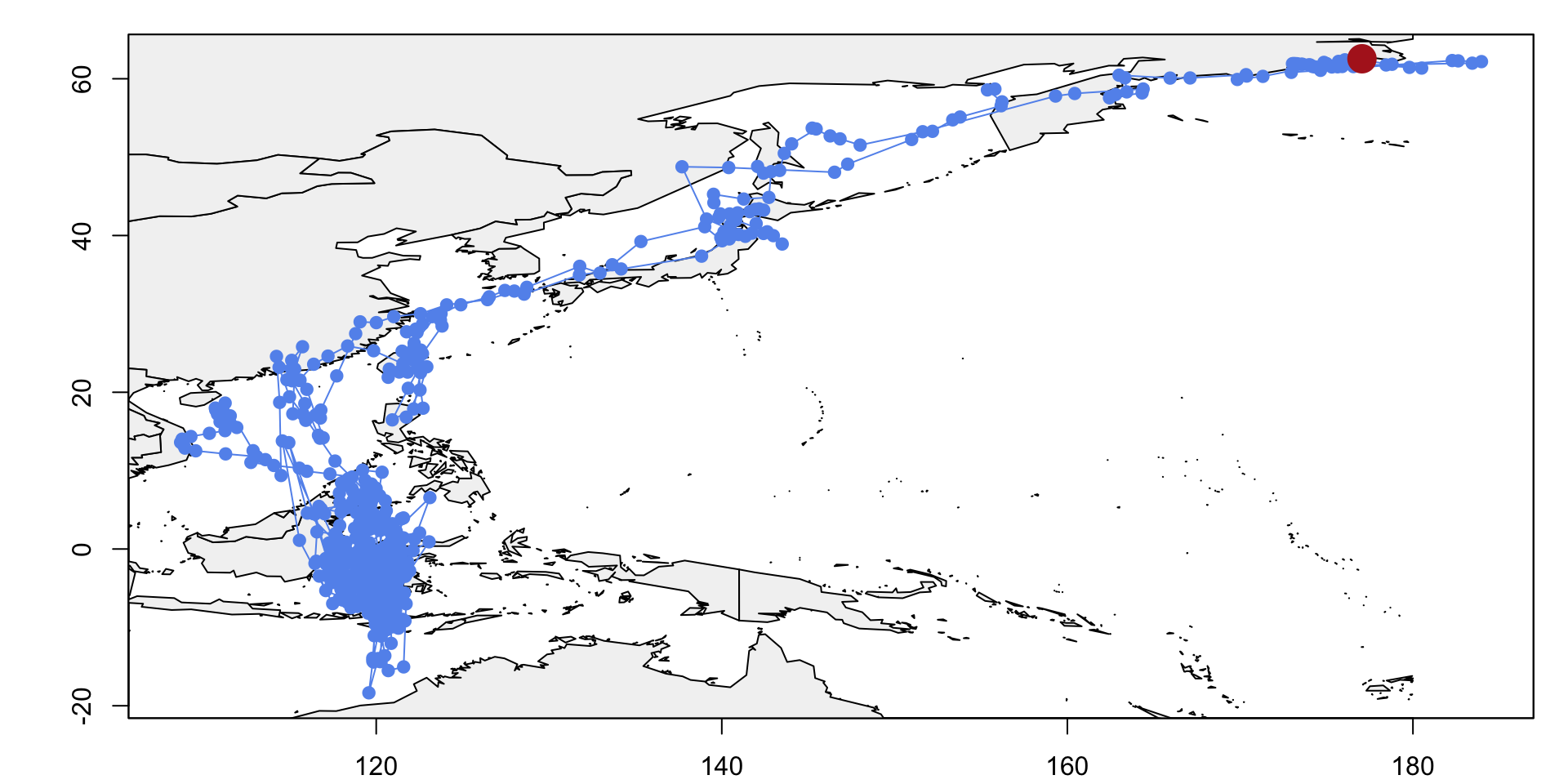

6 Flight R

Now that we have a basic flight track, we can process this data further to generate a track that is based on an algorithm that uses particle filter techniques to provide a flight path with increased accuracy and less noise. The FlightR package provides such an approach to the filtering problem. This consists of estimating the internal states in a dynamical process (the flight path) when partial observations are made, and random perturbations are present in the geolocator data (due to weather) as well as in the dynamical system. First we create the appropriate data structure for the algorithm to run.

# Create dataframe of raw light and datetime records
raw_4_TAGS <- data.frame(
  # Correct date time format
  datetime <- as.POSIXct(raw$Date,tz="UTC"),
  # Raw light data
  light    <- raw$Light)

# Create FlightR file of flight format
FlightR.data <- twGeos2TAGS(raw = raw_4_TAGS, 
                            twl = twl,
                            threshold = 2, 
                            filename = "tages_phal.csv")

# Load and process tags format file
tags_csv <- read_csv("Documents/GitHub/ComputationalEcology/tages_phal.csv")
tags_csv <- tags_csv %>% na.omit()
#write_csv(tags_csv,"tags_clean.csv")

6.1 Calibration

We can use the FlightR package to calibrate via a technique known as template fit⁴. Here the linear relationship (on a log-log scale) between the recorded light levels of a known location and the theoretical light level of that location are used to estimate the angle of the sun, which in turn gives a geospatial location.

# Set-up calibration period
Calibration.periods<-data.frame(
        calibration.start=as.POSIXct("2016-07-04"),
        calibration.stop =as.POSIXct("2016-07-22"),
        lon=177.05, 
        lat=62.55) 

print(Calibration.periods)

# Create calibration object
Calibration <- make.calibration(tags.data, 
                                Calibration.periods,
                                plot.each = F,
                                plot.final = F)

6.2 Assign spatial extent

Before we run the FlightR model, we need to make an estimate as to where we expect the tracked bird will fly, and then assign a spaital grid, within which a model will assign the probability that the bird was present.

# Assign spatial extent
Grid<-make.grid(
  # Assign overall bounding box
  # Use preliminary track from above
  left=100, bottom=-20, right=190, top=70,
  # Can fly over water
  distance.from.land.allowed.to.use=c(-Inf, Inf),
  # Cannot stay further than 30km in land
  distance.from.land.allowed.to.stay=c(-30, Inf))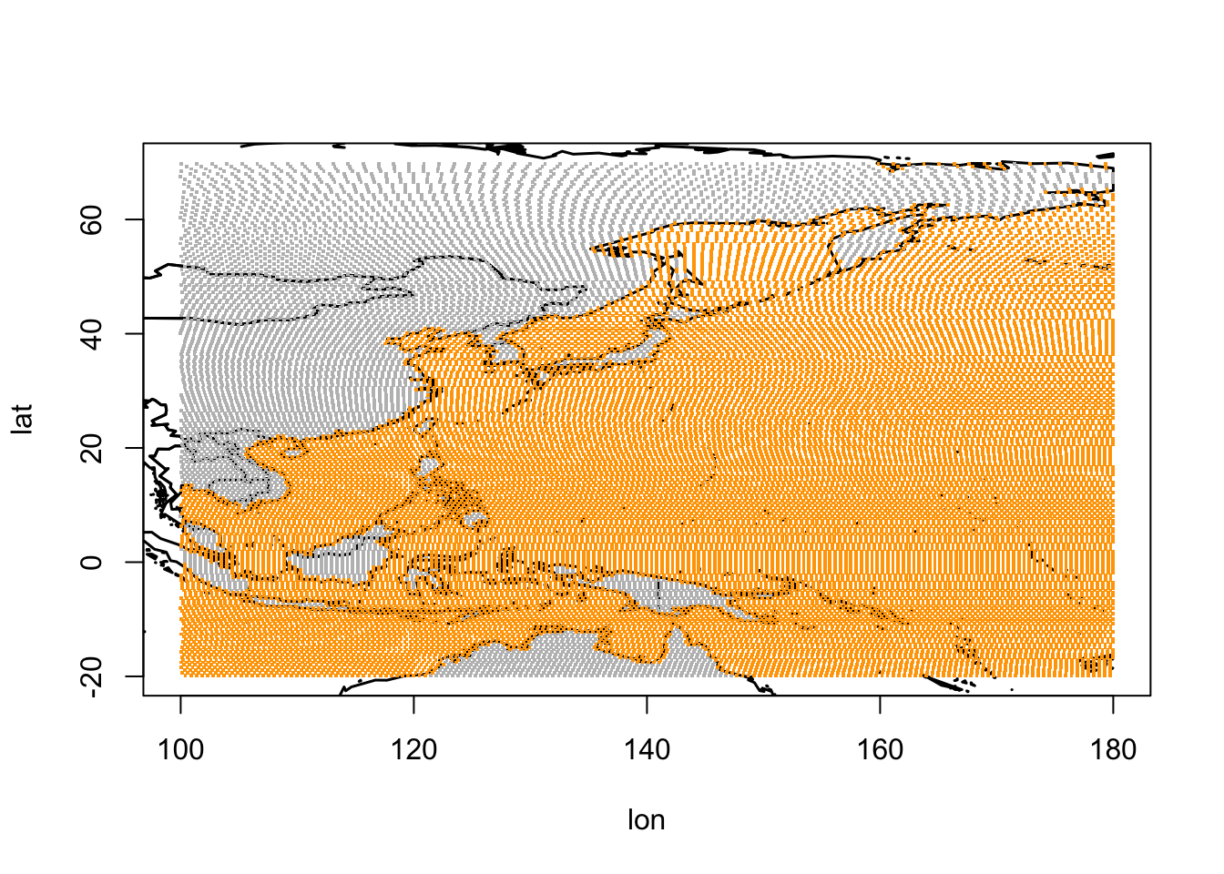

In the above map, yellow shows where we think BA055 will stay/rest and the grey is where the bird may fly.

6.3 Prepare model run

We now combine the various objects we’ve created:

Detected twilight events - tags.data
Spatial extent - Grid
Initial location - Calibration.periods
Calibration parameters - Calibration

And compile a prerun.object. This is then used subsequently to drive the full flight path simulation.

# Prepare the model for execution
# Takes around 15 minutes to run!
all.in <- make.prerun.object(
  # Twilight data
  Proc.data = tags.data, 
  # Spatial extent
  Grid = Grid, 
  # Release location
  start=c(lon.calib, lat.calib),
  # Calibration object
  Calibration=Calibration, 
  # Prior for mean distance travelled (km) between twilights
  M.mean=300)

# Save pre run results
saveRDS(all.in, "BA055_FlightRCalib.RData")

6.4 Particle filter run

Now we are ready to execute a full model run.

# ~ 45 min run time
Result<-run.particle.filter(
  # Pre run object results
  all.in, 
  # Dedicate all threads but 1
  threads=-1,
  # Number of particles in run
  nParticles=1e6, 
  # The bird returned to the same location
  known.last=T,
  # What is the precision of last location
  precision.sd=25, 
  # Ignore outlieers
  check.outliers=F,
  # Maximum distance flown between twilights
  b = 300,
  # Plot results,
  plot = T)

# Save the results of the model run
saveRDS(Result, file="Result.BA055.RData")

7 Discussion

Now we can look at how the longitude and latitude of BA055 flight path changes over time. As the Red Phallarope is known to be a pelagic bird, we can see that BA055 spends the majority of its time over wintering around the equatorial waters east of Indonesia. It has also been recorded as regular visitor within the seas west of New Guinea⁵, where the warm tropical water provides significant foraging grounds for the over wintering birds.

plot_lon_lat(Result)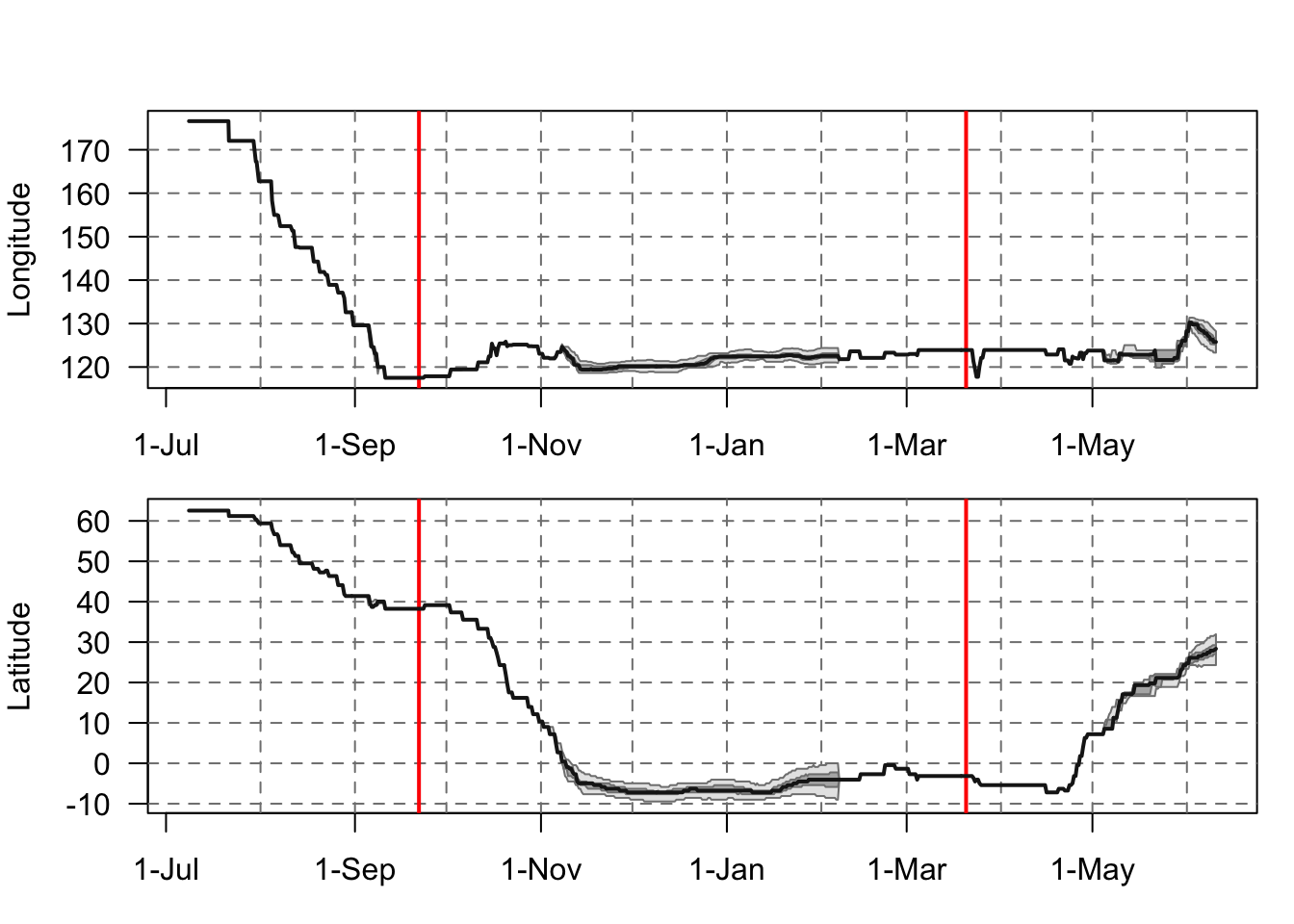

Finally, we can plot a picture of the overall flight path using the Google Maps API. This track presents a cleaner view with less noise as the particle filter algorithm was able to remove the random noise associated with the geologging. Each point represents the most probable latitude and logitude at each twilight. Note, the coloured doughnut is a key for the month of the year.

map.FLightR.ggmap(Result = Result, 
                  seasonal.donut.location = "bottomright")

8 References

Tong Mu , Pavel S. Tomkovich, Egor Y. Loktionov, Evgeny E. Syroechkovskiy, David S. Wilcove: Migratory routes of Red-necked Phalaropes Phalaropus lobatus breeding in southern Chukotka revealed by geolocators.↩
Lisovski, S., Bauer, S., Briedis, M., Davidson, S.C., Dhanjal-Adams, K.L., Hallworth, M.T., Karagicheva, J., Meier, C.M., Merkel, B., Ouwehand, J., Pedersen, L., Rakhimberdiev, E., Roberto-Charron, A., Seavy, N.E., Sumner, M.D., Taylor, C.M., Wotherspoon, S.J. & E.S. Bridge (2019) Light-Level Geolocator Analyses: A user’s guide. Journal of Animal Ecology.↩
Hill, C. & Braun, M.J. (2001) Geolocation by light level - the next step: Latitude. In: Electronic Tagging and Tracking in Marine Fisheries (eds J.R. Sibert & J. Nielsen), pp. 315-330. Kluwer Academic Publishers, The Netherlands.↩
Ekstrom, P. (2007). Error measures for template-fit geolocation based on light. Deep Sea Research Part II: Topical Studies in Oceanography, 54, 392–403.↩
Taufiqurrahman, I (2015). Red-necked phalarope Phalaropus lobatus in west papuan waters, Indonesia↩

Phalaropus lobatus - Migration tracking