Species abundance analysis
1 Introduction
Geostatistics is the area of statistics used to analyze and predict the values associated with spatial or spatiotemporal processes. It incorporates the spatial (and in some cases temporal) coordinates of data within the analyses. Geostatistics attempts to fit a stochastic process to the known locations of a phenomenon and associated covariates, inorder to produce a model that can be used for making wider predictions across space and time.
Here we use a dataset of species observation locations within the Naboisho conservancy in Kenya. In this example we want to ask the question how is Zebra abudaance distributed across the conservancy for a given date range, and we will use geostatistical techniques to determine this.
We start by loading the relevant libraries and data.
# Load libraries
library(tidyr)
library(dplyr)
library(sf)
library(ggplot2)
library(geosphere)
library(lwgeom)
library(PrevMap)
library(raster)

# Set filename of raw csv to load
rm(list = ls())
setwd("/Users/anthony/Documents/GitHub/ComputationalEcology/")
survey <- readRDS("data_analysis_files/naboisho/clean_survey.RData")
2 Visualising the data
We can visualise all the data that has been collected within the Naboisho conservancy data set. The chart below shows the observer location, for each given species that was recorded. A compass and laser was used for each observation, to determine the observed species location relative to the observer.
# Add sf POINTs to dataframe for coords
survey <- survey %>%
  # Remove observations with no long, lat data
  filter(!is.na(lat) & !is.na(long)) %>%
  # Create sf points with WGS84
  st_as_sf(coords = c("long", "lat"), crs = 4326, remove = F)

# Plot overall data set
survey %>%
  ggplot() +
    geom_point(aes(x=long, y=lat)) +
    facet_wrap(~transect, scale = "free") +
    theme_bw() +
  ggtitle("Nabosiho transect observer locations")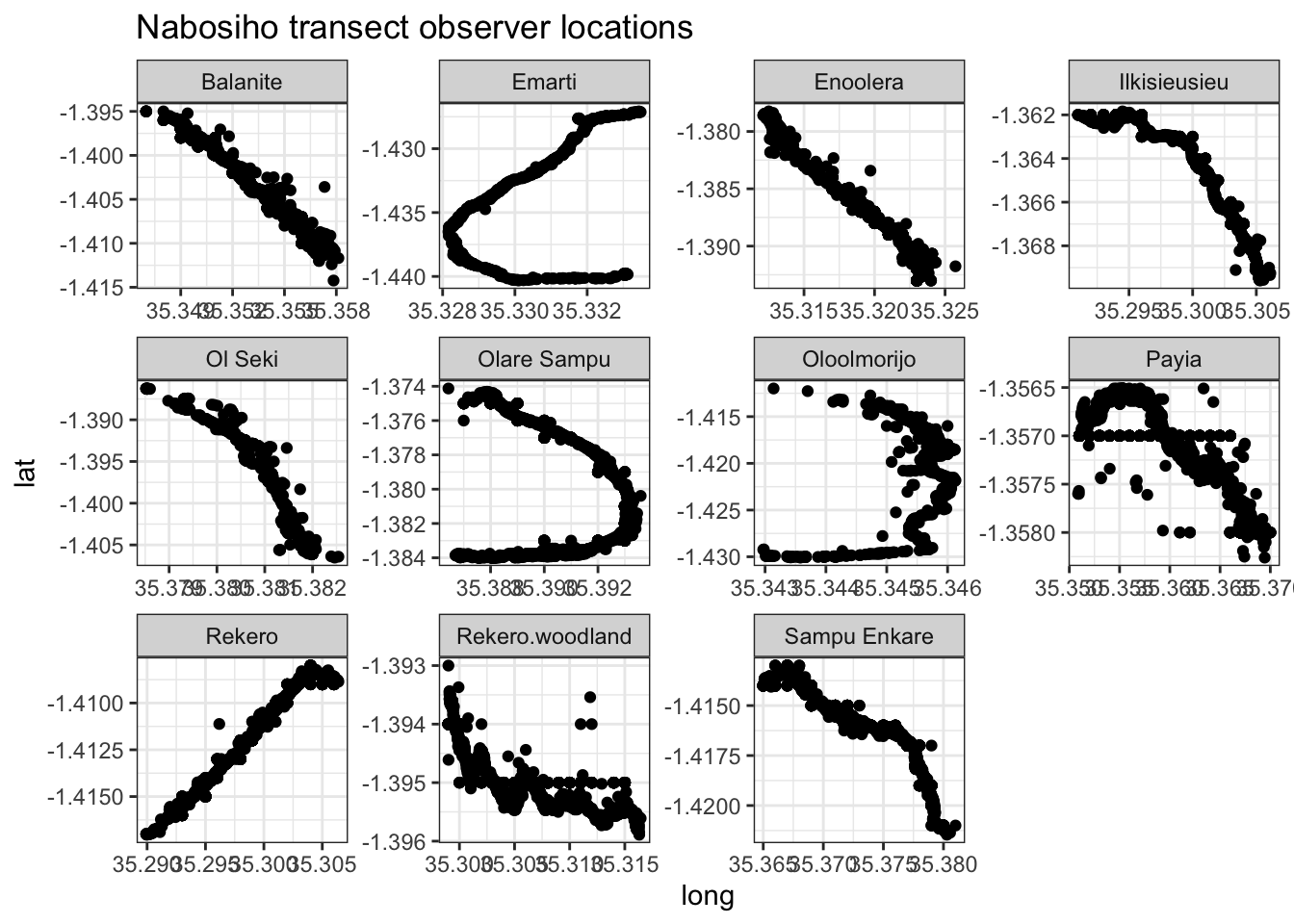
2.1 Generating species locations
Now we need to generate the coordinates of all species, given the observer location (long, lat), distance between species and observer and compass bearing.
species_locations <- geosphere::destPoint(
  # drop sf geometry and select vector of observer locations
  p = survey %>% st_drop_geometry() %>% dplyr::select(long,lat),
  # vector of bearings from observer to observations
  b = survey$Compass.Bearing,
  # vector of distance in meters between observer and observation
  d = survey$Distance..m.) %>%
  # Convert new destinations to a dataframe
  as.data.frame() %>%
  # Create sf point from species location
  st_as_sf(coords = c('lon', 'lat'), crs = 4326, remove = F) %>%
  # Project into planar coordinates for Kenya
  st_transform(32636) %>%
  # Bind with relevant survey data
  cbind(
    survey %>% dplyr::select(size, Region.Label, transect, species, year, month)) %>%
  distinct(.keep_all=T)

# Add Easting/Northing references to datframe
species_locations <- species_locations %>%
  st_coordinates() %>%
  cbind(species_locations) %>%
  rename (easting = X,
          northing = Y) %>%
  st_drop_geometry()

# Plot all species locations
species_locations %>%
  ggplot() +
    geom_point(aes(x=lon, y=lat)) +
    theme_bw() +
    ggtitle("Species locations across all Naboisho data")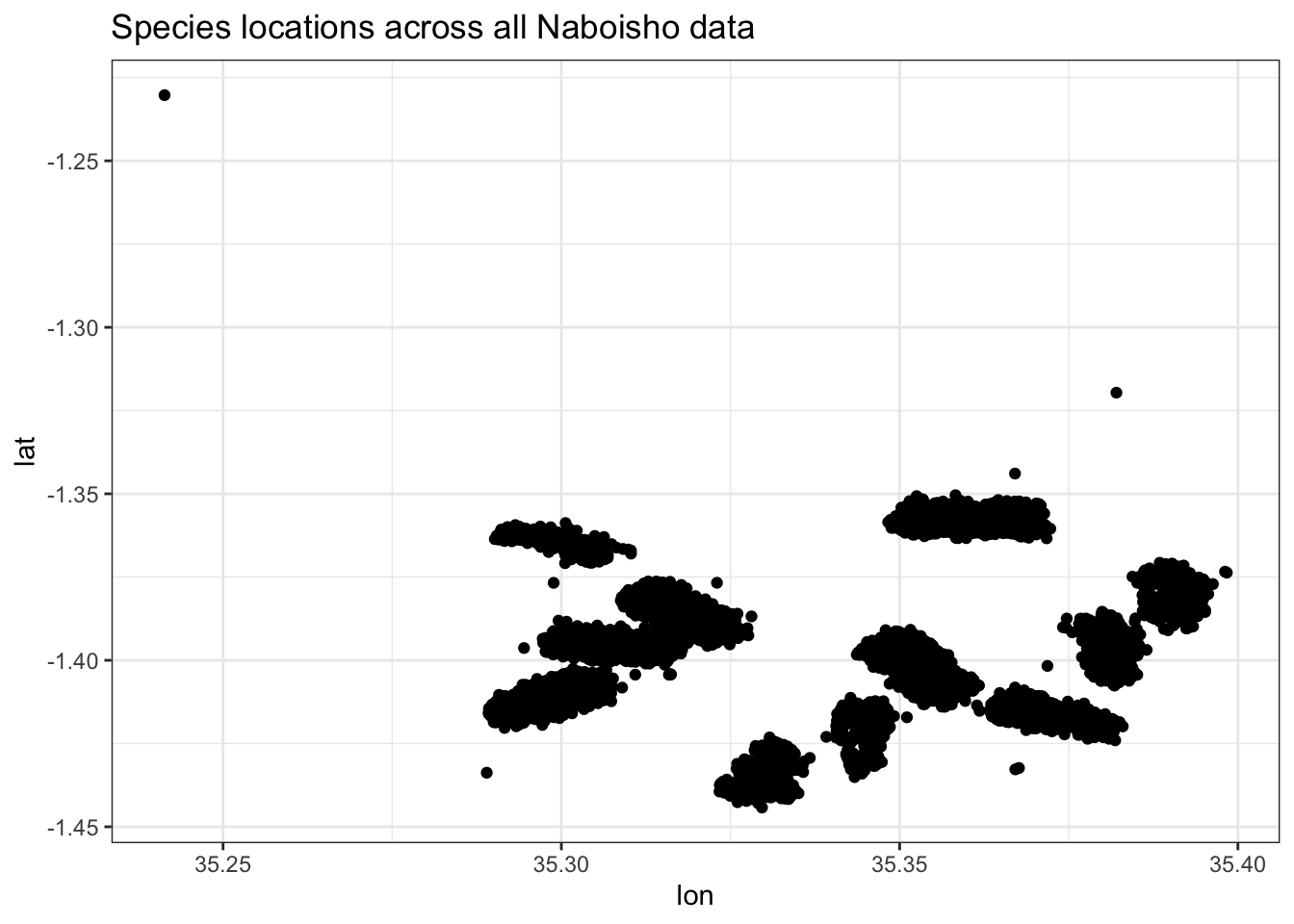
Looks like we have a few outliers, so let’s remove them. And now we can plot locations of species across all dates.
# Remove the outlier
species_locations <- species_locations %>%
  filter(lat < -1.325) %>%
  # Remove species marked as None
  filter(species != "None")

#Replot
species_locations %>%
    ggplot() +
    geom_point(aes(x=lon, y=lat)) +
    theme_bw() +
    facet_wrap(~species) +
    ggtitle("Species locations across all Naboisho data, all years")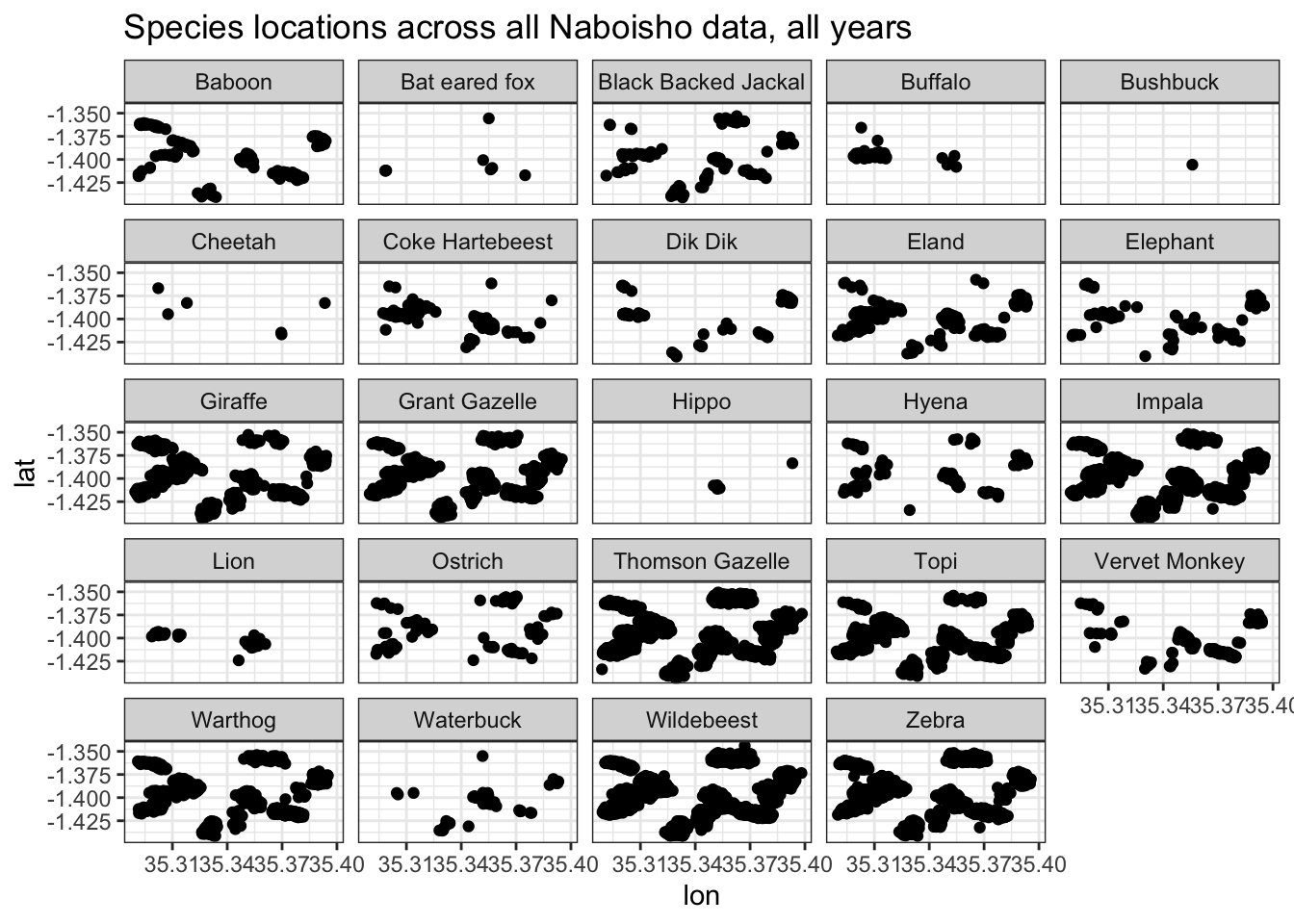
# Generate bounding box for Naboisho in WGS84
naboisho_bbox <- st_bbox(species_locations$geometry)
3 Spatial Zebra observations in time
We want to select Zebra to generate a spatial abundance estimation. Our spatial model assumes that the random process within it is a stationary process. That is, the statistical properties within it are applicable across the entire spatial domain acroos the given timescale for which the observations were made. Therefore we should select Zebra observations from a particular point in time. Below we choose observations from July 2018 only.
# Create target dataset
zebra <- species_locations %>%
  filter(species == "Zebra") %>%
  filter(year == 2018) %>%
  filter(month == "Jul") %>%
  # Keep only the location, count and covariates
  dplyr::select(easting, northing, size, Region.Label, transect)

# Plot Zebra in July of 2019
zebra %>%
  ggplot() +
  geom_point(aes(x=easting, y=northing, size=size)) +
  theme_bw() +
  ggtitle("Zebra group sizes observed in Naboisho, in July 2018")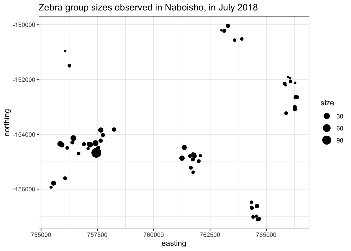
The plot above shows Zebra locations from a survey within the Naboisho conservancy as of July 2018. Note the size of the dot shows the size of the Zebra heard observed.
4 Adding NDVI as a model covariate
Before we generate our spatial model, we can generate a Normalised Difference Vegetation Index (NDVI) for the Naboisho conservancy. NDVI quantifies the degree of vegetation spatially by measuring the difference between reflected near-infrared (which vegetation reflects) and red light (which vegetation absorbs). We can use this spatial information as a covariate and can therefore explore the association of Zebra abundance with the degree of vegetation.
To generate an NDVI index we use a Landsat satellite raster from July 2018. For each 30m x 30m cell within the raster image, we process the NIR and Red light values to generate an NDVI value. The results is a set of coordinates in space, each of which with a value between -1 and 1. A value of +1 represents represents dense green vegetation and values around 0 or less represent urbanised developments.
# Load NDVI of naboisho for July 2019
ndvi_r <- raster("data_analysis_files/naboisho/naboisho_ndvi_cropped") %>%
  # Downsample raster to 120m x 120m cells
  aggregate(fact=8, fun=mean)
# Plot NDVI of Naboisho study region
plot(ndvi_r, main="Naboisho NDVI, July 2018")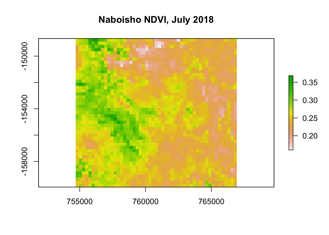
# Extract NDVI for each observation and bind to observation data
zebra <- ndvi_r %>%
  raster::extract(zebra[1:2]) %>%
  cbind(zebra) %>%
  dplyr::rename(ndvi = ".")
5 Fitting a variogram
A variogram is a fundamental building block of geostatistics. Its purpose is to capture the spatial continuity and structure within a dataset. In our Zebra example, a variogram will give a measure of how two different observations vary in abundance as a function of distance between them. To calculate it, a function selects pairs of points (at a different distances, known as lag) from a dataset, and measures the variability between them. We can use the r package gstat to fit and plot an empirical variogram.
library(gstat)
coordinates(zebra) <- ~ easting + northing

# Generate sample variogram values for species location data
species_vgm <- gstat::variogram(size ~ ndvi, zebra)
# Fit model
species_fit <- fit.variogram(species_vgm, model=vgm(1, "Sph", 900,1))
#species_fit <- fit.variogram(species_vgm, model=vgm(5, "Sph", 8,2))
# Show model parameters
species_fit
## model psill range
## 1 Nug 183.8316 0.0000
## 2 Sph 162.2805 709.7361# Plot the model fit
plot(species_vgm, species_fit, main = "Variogram for Zebra")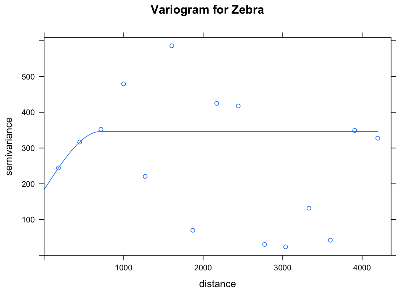
There are three key parameters that describe the variogram:
- nugget : the point at which the variograme hits the y axis.
- sill : the limit of the variogram tending to infinite lag distances
- range : the distance in which the difference of the variogram from the sill becomes negligible
The range is the key parameter that helps fit our geospatial model.
6 A spatial abundance model
In order to generate a spatial abundance model from the Naboisho Zebra data, we use the r package PrevMap 1. PreMap is used to analyse spatially referenced prevalance data, and uses classical maximum likelihod estimation as well as Bayesian inference, in order to estate parameters of spatial models. To model species abundance counts in space, we use a poission model that has its parameters estimated by using a Monte Carlo maximum likelihood estimator. We take the output of the variogram model to initiate parameterisation of the estimator, as follows.
fit.LA <- glgm.LA(size ~ ndvi,
                  coords = ~ I(easting) + I(northing),
                  kappa=0.5,
                  start.cov.pars = species_fit$range[2],
                  fixed.rel.nugget = 0.0,
                  data=zebra,
                  family="Poisson")

# Specify control parameters for Monte Carlo Maximum Likelihood simulation
par0 <- coef(fit.LA)
c.mcmc <- control.mcmc.MCML(n.sim=10000,
                            burnin=2000,
                            thin=8)

# Run the MCML
fit.MCML <- poisson.log.MCML(size ~ ndvi,
                             # Specify control parameters
                             control.mcmc = c.mcmc,
                             par0=par0,
                             # Specify coordinates
                             coords=~I(easting)+I(northing),
                             kappa=0.5,
                             start.cov.pars = species_fit$range[2],
                             fixed.rel.nugget = 0,
                             data=zebra,
                             method="nlminb")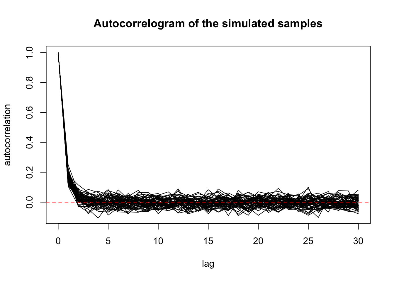
summary(fit.MCML)7 Model prediction
Now we have estimated the parameters for our model, we can make a spatial abundance prediction. Inorder to make a prediction, we need to make a prediction grid that includes the NDVI covariate data that we generated earlier. This will drive the prediction of the response variable (Zebra abundance) within each cell of the prediction grid.
pred_grid <- ndvi_r %>%
  # Convert raster to vector of points
  rasterToPoints() %>%
  as.data.frame() %>%
  rename(easting = x,
         northing = y,
         ndvi = layer)
Now we can make a prediction.
# Generate prediction data
pred.MCML <- spatial.pred.poisson.MCML(fit.MCML,
                                       grid.pred = pred_grid,
                                       control.mcmc = c.mcmc,
                                       type = "marginal",
                                       predictors = pred_grid,
                                       standard.errors = T,
                                       plot.correlogram = T)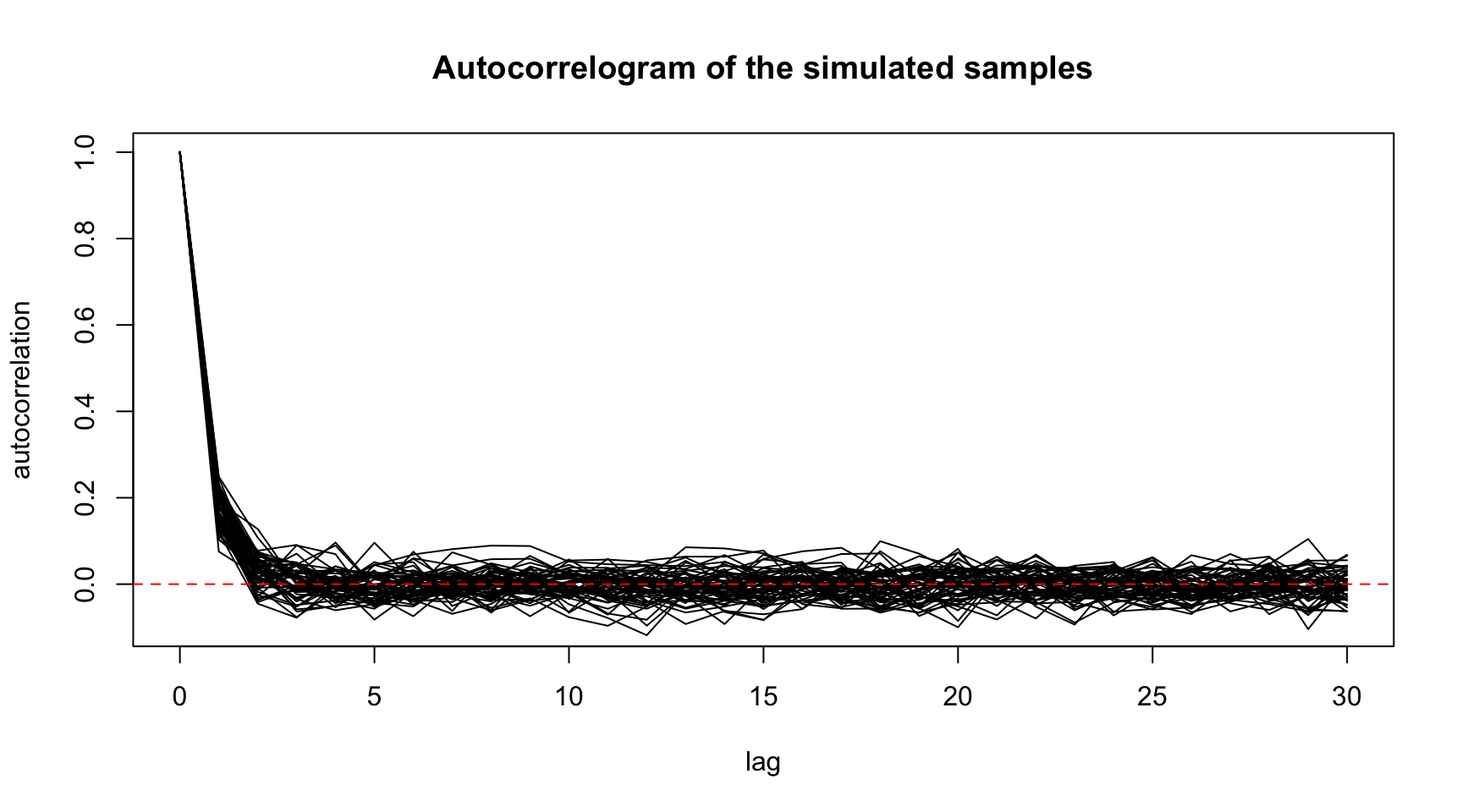
We can plot the spatial distribution of the mean exponential abundance together with the variance.
predictions <- cbind(
  # Select predictions
  exp_pred = pred.MCML$exponential$predictions,
  # Select standard errors
  std_err = pred.MCML$exponential$standard.errors,
  # Specifiy the prediction grid
  pred_grid %>% dplyr::select(easting,northing))

# Now plot predictions
predictions %>%
  ggplot(aes(x=easting, y=northing)) +
  geom_tile(aes(fill=exp_pred)) +
  coord_equal() +
  scale_fill_viridis_c() +
  theme_bw() +
  ggtitle("Predicted Zebra abundance, Naboisho, July 2018")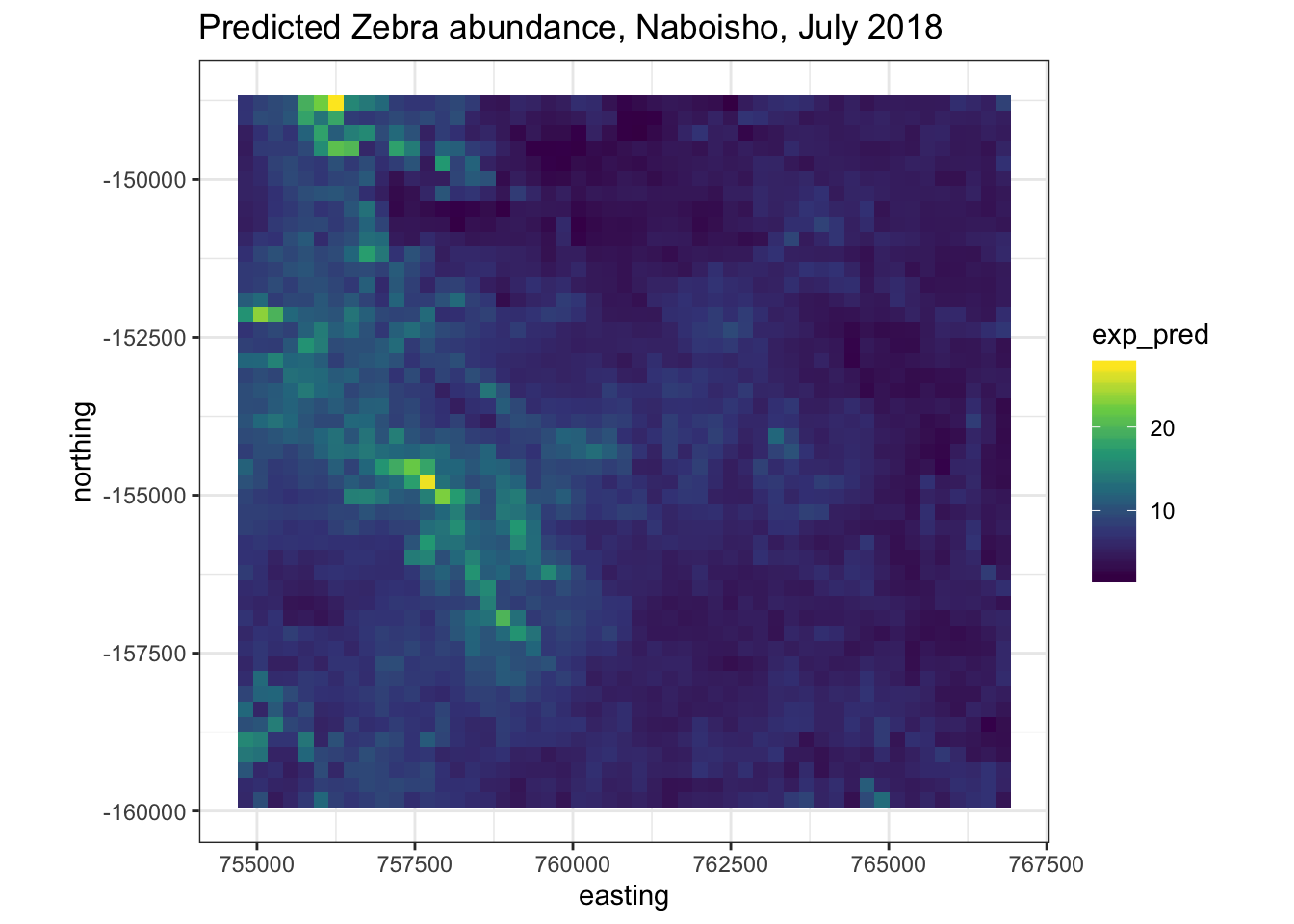
# Show details of model fit summary
summary(fit.MCML)
## Geostatistical Poisson model
## Call:
## poisson.log.MCML(formula = size ~ ndvi, coords = ~I(easting) +
## I(northing), data = zebra, par0 = par0, control.mcmc = c.mcmc,
## kappa = 0.5, fixed.rel.nugget = 0, start.cov.pars = species_fit$range[2],
## method = "nlminb")
##
## Estimate StdErr z.value p.value
## (Intercept) -1.5184 0.8429 -1.8014 0.07164 .
## ndvi 12.4003 3.1621 3.9216 8.797e-05 ***
## ---
## Signif. codes: 0 '***' 0.001 '**' 0.01 '*' 0.05 '.' 0.1 ' ' 1
##
## Objective function: 0.00401485
##
## Covariance parameters Matern function
## (fixed relative variance tau^2/sigma^2= 0)
## Estimate StdErr
## log(sigma^2) -0.66092 2.4220e-01
## log(phi) 0.39341 1.0861e+05
##
## Legend:
## sigma^2 = variance of the Gaussian process
## phi = scale of the spatial correlationCalculate the overall population density per km2
# Calculate total number
total_count = sum(log(pred.MCML$exponential$predictions))
total_count
## [1] 4418.931# Calculate survey area in km2
survey_area = nrow(ndvi_r) * ncol(ndvi_r) * xres(ndvi_r)/1000 * yres(ndvi_r)/1000
survey_area## [1] 138.0672# Calculate average density per km2
density = total_count / survey_area
density## [1] 32.005658 Discussion
In conservation ecology it is important to understand how the abundance of given species responds to covariates such as habitat or vegetation, in time and space. Geostastics is a technique is a tool that can help the ecologist understand this question. The technique was first developed to improve understanding of how ore grades varied across open cast mines in South Africa2. But the underlying theory of spatial estimation is particularly relevant to landscape conservation ecologists.
9 References
Giorgi, E., Diggle, P. J. (2016). PrevMap: an R package for prevalence mapping. Journal of Statistical Software. In press↩